Introduction to K-Nearest Neighbor
KNN is a supervised learning algorithm and uses a training sample from the dataset, which classifies groups into different classes. It is a classifier used to predict the level of an unknown point (observation) and does this by measuring the points nearest to the unknown point. It works well in measuring the differences between multiple classes that are complex and hard to detect. KNN is considered a simple classification and regression algorithm. In classification, new data points are grouped into a given class, while in regression, a new data point is labeled based on the average value of k nearest neighbor. KNN is a “lazy learner” because it doesn’t learn more than the training data
Distance measurements used in KNN?
One of the KNN algorithm’s only freedoms where we can play around and pick different things resulting in different classifiers and performance is the algorithm’s distance parameter. The Euclidean distance is the default measure. A useful application for numeric attributes with continuous data. Symmetric, spherical, and treats all dimensions equally. Sensitive to extreme differences (outliers) in single variables. The Minkowski distance is a p-norm or generalization of the Euclidean distance. KNN can also do the Manhattan distance (adds the difference across each coordinate point) by setting p =1 or set p=0 for Hamming distance (suitable for categorical attributes). Also found the Kullback-Leibler (KL) divergence for histograms (is asymmetrical) and mentions a custom distance measurement called BM25 for text.
Applications of the KNN Algorithm
Applications using KNN are facial recognition, character recognition in video and images. Traffic monitoring systems that stream video of traffic patterns and maps out predictions. Another application is a recommender system for consumer products that predicts products for consumers. The biomedical industry also uses KNN to predict biologically related occurrences such as tumor detection or onset of diabetes. Another area is the scientific and environmental analysis of various elements occurring at a site.
Pros and Cons of using the K-Nearest Neighbor Algorithm
Pro:
The KNN is simple and effective, according to the experts, and said to be impressive for a simpler method. The decision line can be any shape versus a straight line in other classifiers, and this is beneficial for complex, multiple groups of data all clustered together. The algorithm always separates the training set precisely because of the “noise cell” made by the decision boundary around the points. It’s non-linear and reflects classes well. There is a lot of freedom to fit the training data. The distance measure is a benefit because we can choose one appropriate to the data’s complexity or type of data. There is no over/under fitting of the model, as the k value is adjusted appropriately.
Con:
Data needs scaling, which is adjusted before running the data, which adds a step to the process. Watch for units of measurement like the height of a tree compared to the width of its leaves. Meters verse mm can severely alter the decision boundary. If the data is overly noisy with no clear definition between classes, KNN may not work at its best. The computation cost is high and will use resources; thus, speed can be a factor. Outliers and mislabeled points can alter the decision boundary significantly. Missing values need to be filled in with something and can’t be left empty – use imputation or remove data. We don’t want these small changes to the training set to affect the classifier problem. There is no notion of prior states – no confidence in the class prior. Making the k value too big the algorithm will classify everything as the most probable. Making k too small leads to unstable decision boundaries and high variability. The small changes in the training set magnify changes in classification.
K-Nearest Neighbor Example
This project example uses the UCI data sets (https://archive.ics.uci.edu/ml/datasets/Heart+Disease) “Heart-Disease” and specifically the “processed.cleveland.data” for this analysis. The data has fourteen attributes. We note one of the attributes (variables), num is the predicted attribute for this KNN model exercise. Eight attributes are categorical, and five attributes are numerical. We will create dummy variables for the eight categorical and scale the five numeric variables. The predictor attribute is a factor. And is changed to either No presence of the angiographic disease or Yes for the angiographic disease.
Load the Libraries
library(tidyverse)
library(caret)
library(pROC)
library(corrplot)
library(gridExtra)
library(psych)
Load the Dataset
HD = read_csv("https://archive.ics.uci.edu/ml/machine-learning-databases/heart-disease/processed.cleveland.data",
            col_names = c("age","sex","cp","trestbps","chol",
                          "fbs","restecg","thalach","exang","oldspeak",
                          "slope","ca","thal","num"))
Dataset Description
Attribute Information:
age(in years)sex(1=male, 0=female)cp(chest pain type: 1:=typical angina, 2:=atypical angina, 3=non-anginal pain, 4=asymptomatic)trestbps(resting blood pressure in mm Hg on admission to the hospital)chol(serum cholesterol in mg/dl)fbs(fasting blood sugar > 120 mg/dl, 1 = true; 0 = false)restecg(resting electrocardiograph results, 0=normal, 1=ST-T wave abnormality, T wave inversions and/or ST elevation or depression of > 0.05 mV, 2=showing probable or definite left ventricular hypertrophy by Estes’ criteria)thalach(maximum heart rate achieved)exang(exercise induced angina, 1 = yes; 0 = no)oldpeak(ST depression induced by exercise relative to rest)slope(the slope of the peak exercise ST segment, 1=upsloping, 2= flat, 3=downslopingca(number of major vessels (0-3) colored by flourosopy)thal(3 = normal; 6 = fixed defect; 7 = reversible defect)num(the predicted attribute, diagnosis of heart disease, angiographic disease status, 0: < 50% diameter narrowing, 1: > 50% diameter narrowing)
Data Summary
## Rows: 303
## Columns: 14
## $ age      <dbl> 63, 67, 67, 37, 41, 56, 62, 57, 63, 53, 57, 56, 56, 44, 52...
## $ sex      <dbl> 1, 1, 1, 1, 0, 1, 0, 0, 1, 1, 1, 0, 1, 1, 1, 1, 1, 1, 0, 1...
## $ cp       <dbl> 1, 4, 4, 3, 2, 2, 4, 4, 4, 4, 4, 2, 3, 2, 3, 3, 2, 4, 3, 2...
## $ trestbps <dbl> 145, 160, 120, 130, 130, 120, 140, 120, 130, 140, 140, 140...
## $ chol     <dbl> 233, 286, 229, 250, 204, 236, 268, 354, 254, 203, 192, 294...
## $ fbs      <dbl> 1, 0, 0, 0, 0, 0, 0, 0, 0, 1, 0, 0, 1, 0, 1, 0, 0, 0, 0, 0...
## $ restecg  <dbl> 2, 2, 2, 0, 2, 0, 2, 0, 2, 2, 0, 2, 2, 0, 0, 0, 0, 0, 0, 0...
## $ thalach  <dbl> 150, 108, 129, 187, 172, 178, 160, 163, 147, 155, 148, 153...
## $ exang    <dbl> 0, 1, 1, 0, 0, 0, 0, 1, 0, 1, 0, 0, 1, 0, 0, 0, 0, 0, 0, 0...
## $ oldspeak <dbl> 2.3, 1.5, 2.6, 3.5, 1.4, 0.8, 3.6, 0.6, 1.4, 3.1, 0.4, 1.3...
## $ slope    <dbl> 3, 2, 2, 3, 1, 1, 3, 1, 2, 3, 2, 2, 2, 1, 1, 1, 3, 1, 1, 1...
## $ ca       <chr> "0.0", "3.0", "2.0", "0.0", "0.0", "0.0", "2.0", "0.0", "1...
## $ thal     <chr> "6.0", "3.0", "7.0", "3.0", "3.0", "3.0", "3.0", "3.0", "7...
## $ num      <dbl> 0, 2, 1, 0, 0, 0, 3, 0, 2, 1, 0, 0, 2, 0, 0, 0, 1, 0, 0, 0...
Missing values found in thal and ca. Changing the character type to a numeric type, this will replace missing with NA.
HD$thal = as.double(HD$thal)
HD$ca = as.double(HD$ca)
## age sex cp trestbps
## Min. :29.00 Min. :0.0000 Min. :1.000 Min. : 94.0
## 1st Qu.:48.00 1st Qu.:0.0000 1st Qu.:3.000 1st Qu.:120.0
## Median :56.00 Median :1.0000 Median :3.000 Median :130.0
## Mean :54.44 Mean :0.6799 Mean :3.158 Mean :131.7
## 3rd Qu.:61.00 3rd Qu.:1.0000 3rd Qu.:4.000 3rd Qu.:140.0
## Max. :77.00 Max. :1.0000 Max. :4.000 Max. :200.0
##
## chol fbs restecg thalach
## Min. :126.0 Min. :0.0000 Min. :0.0000 Min. : 71.0
## 1st Qu.:211.0 1st Qu.:0.0000 1st Qu.:0.0000 1st Qu.:133.5
## Median :241.0 Median :0.0000 Median :1.0000 Median :153.0
## Mean :246.7 Mean :0.1485 Mean :0.9901 Mean :149.6
## 3rd Qu.:275.0 3rd Qu.:0.0000 3rd Qu.:2.0000 3rd Qu.:166.0
## Max. :564.0 Max. :1.0000 Max. :2.0000 Max. :202.0
##
## exang oldspeak slope ca
## Min. :0.0000 Min. :0.00 Min. :1.000 Min. :0.0000
## 1st Qu.:0.0000 1st Qu.:0.00 1st Qu.:1.000 1st Qu.:0.0000
## Median :0.0000 Median :0.80 Median :2.000 Median :0.0000
## Mean :0.3267 Mean :1.04 Mean :1.601 Mean :0.6722
## 3rd Qu.:1.0000 3rd Qu.:1.60 3rd Qu.:2.000 3rd Qu.:1.0000
## Max. :1.0000 Max. :6.20 Max. :3.000 Max. :3.0000
## NA's :4
## thal num
## Min. :3.000 Min. :0.0000
## 1st Qu.:3.000 1st Qu.:0.0000
## Median :3.000 Median :0.0000
## Mean :4.734 Mean :0.9373
## 3rd Qu.:7.000 3rd Qu.:2.0000
## Max. :7.000 Max. :4.0000
## NA's :2Remove the NA missing values from the data. Four in ca and two in thal.
HD = drop_na(HD)Change those categorical variables to factor type, and these will be re-encoded in later steps.
HD = HD %>% mutate_at(c("cp", "restecg", "slope", "ca", "thal"), as.factor)Correlation Matrix
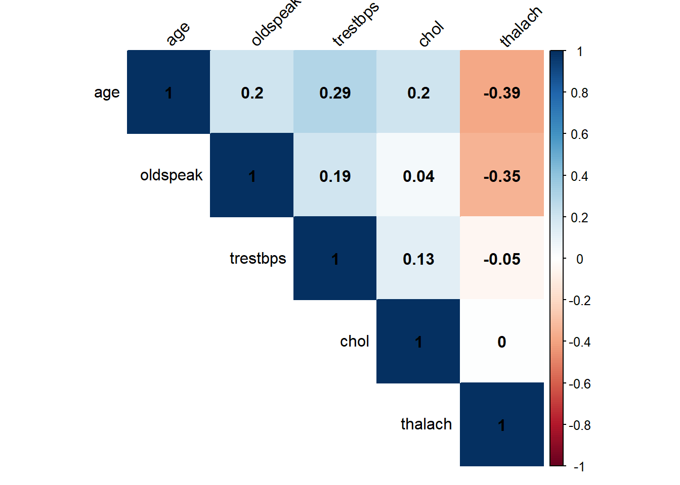
Observations describing the correlation between the numeric variables: age and oldspeak to thalach and trestbps show a weak negative relationship. The remaining variable shows no linear relationship if only slight.
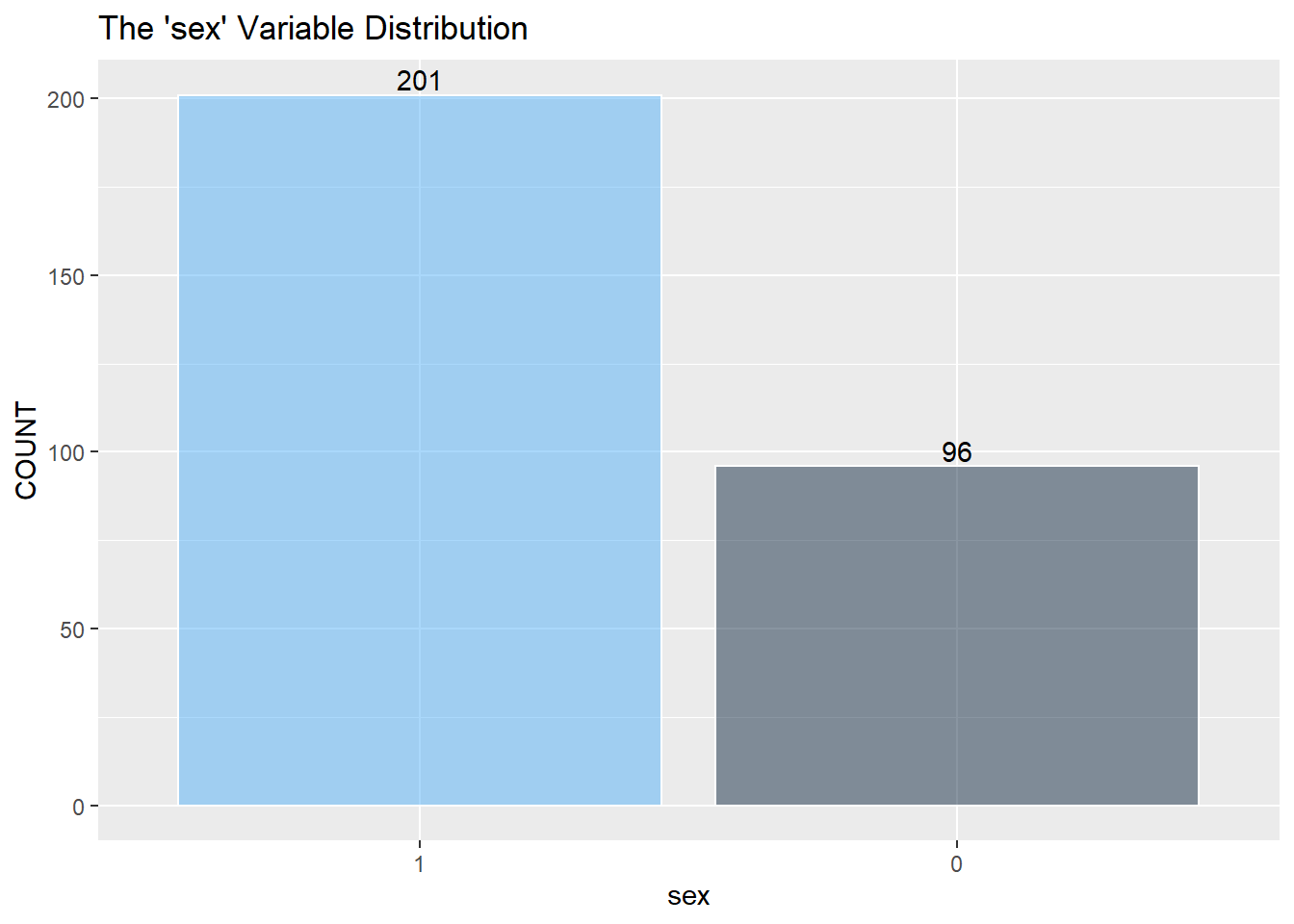
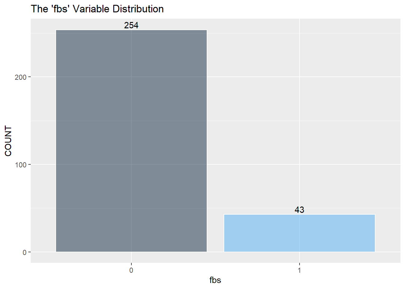
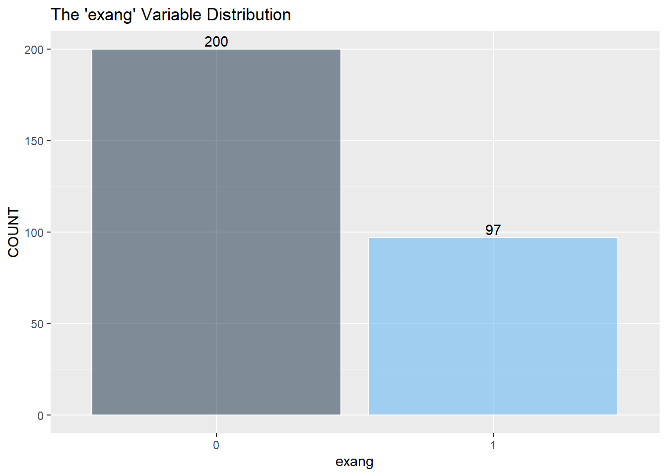
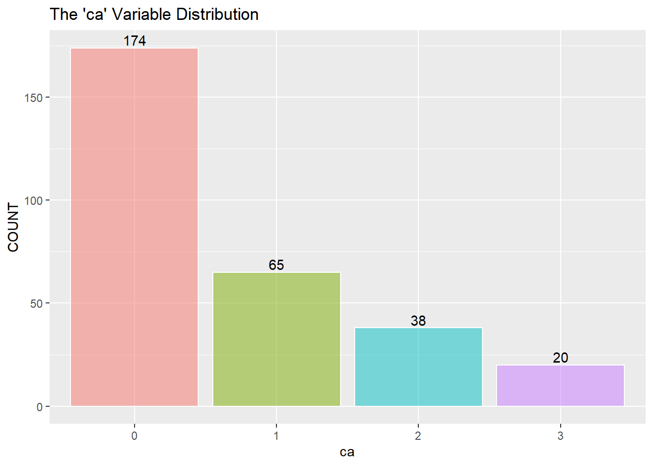
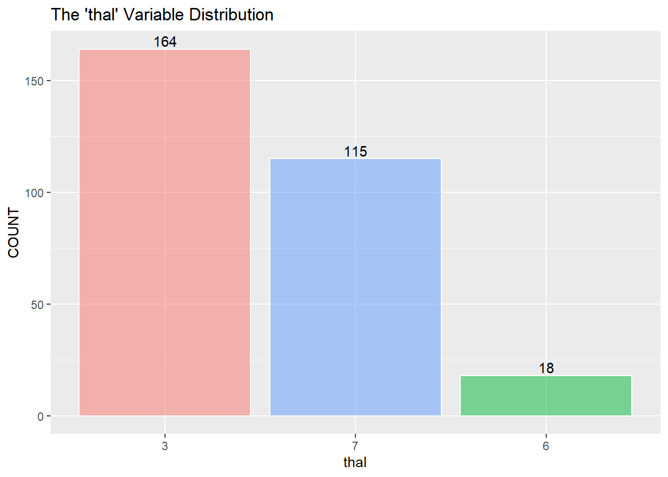
Categorical Variables
Next is a look at the nine categorical variables.

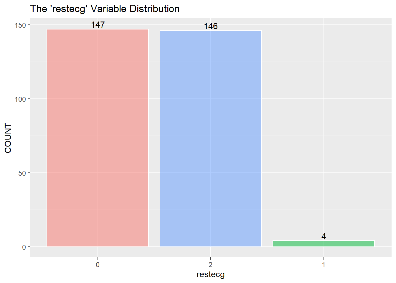
restecg has an imbalance of its three classes. There will be an issue when splitting the training and testing data, and there won’t be enough points representing restecg == 1. It may be best to remove class 1.

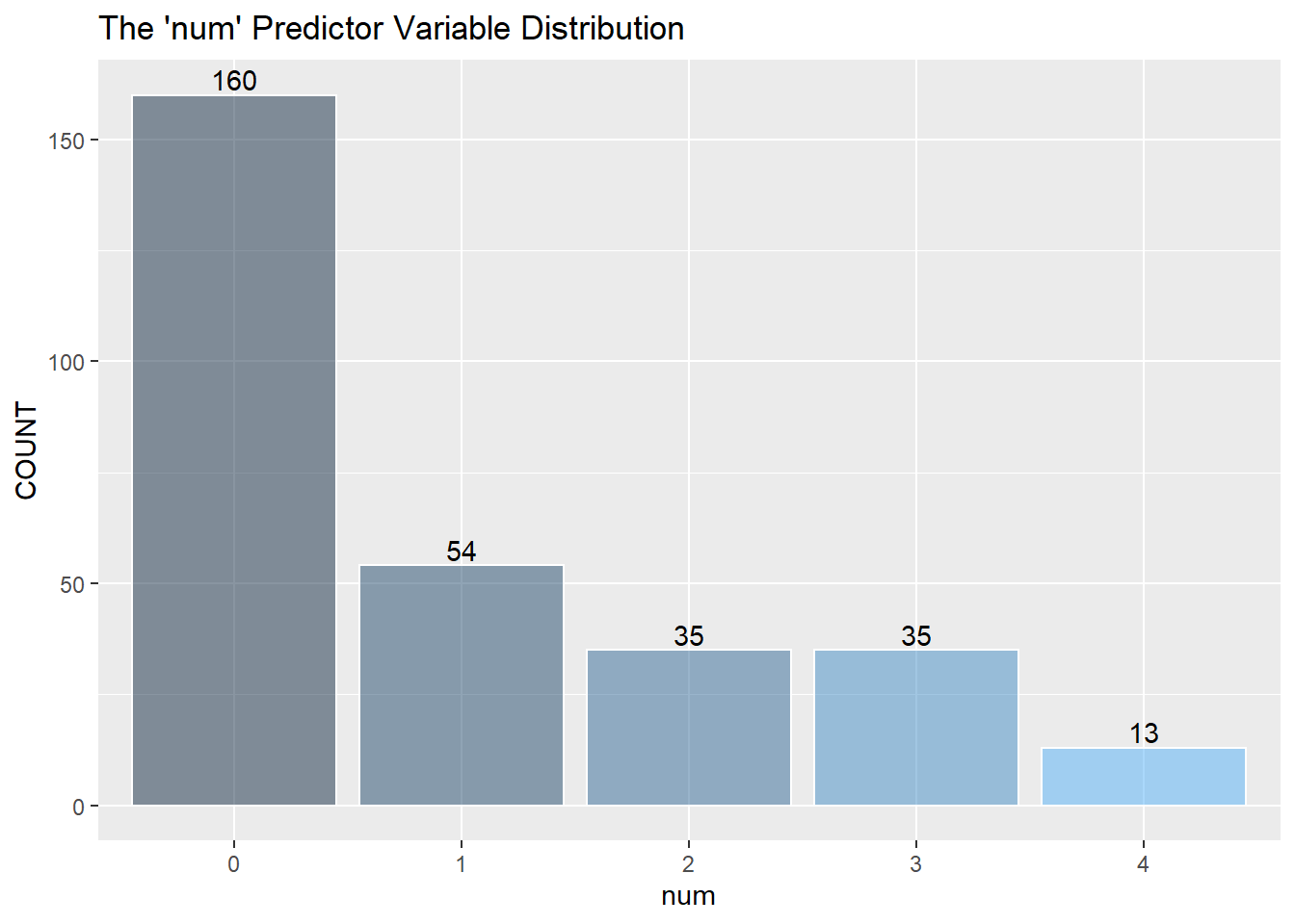
I assume to consolidate the values greater than 0 into the value of 1 and describe 1 as a positive “yes” reading for heart disease. (The information about the data only mentions 0 or 1) I then recode zero and one into “No” and “Yes” as factors for the KNN classifier below.
HD$num[HD$num > 0] = 1
HD$num = recode(HD$num, '0' = "No", '1' = "Yes")
HD$num = factor(HD$num)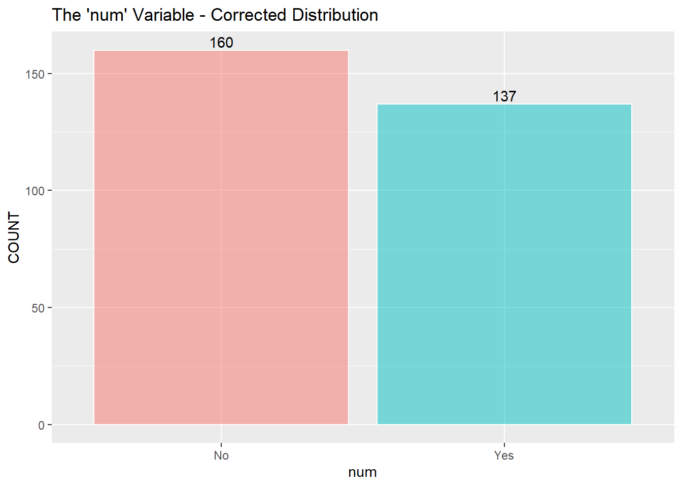
Numeric Variable Summary Statistics
This table shows all of the numeric variables’ statistics. I am looking for outliers, overly skewed distributions, and whether to center the data or not.
| vars | n | mean | sd | median | trimmed | mad | min | max | range | skew | kurtosis | se | Q0.25 | Q0.75 | |
|---|---|---|---|---|---|---|---|---|---|---|---|---|---|---|---|
| age | 1 | 297 | 54.54 | 9.05 | 56.0 | 54.73 | 8.90 | 29 | 77.0 | 48.0 | -0.22 | -0.55 | 0.53 | 48 | 61.0 |
| sex | 2 | 297 | 0.68 | 0.47 | 1.0 | 0.72 | 0.00 | 0 | 1.0 | 1.0 | -0.75 | -1.44 | 0.03 | 0 | 1.0 |
| trestbps | 4 | 297 | 131.69 | 17.76 | 130.0 | 130.48 | 14.83 | 94 | 200.0 | 106.0 | 0.69 | 0.76 | 1.03 | 120 | 140.0 |
| chol | 5 | 297 | 247.35 | 52.00 | 243.0 | 244.70 | 47.44 | 126 | 564.0 | 438.0 | 1.11 | 4.30 | 3.02 | 211 | 276.0 |
| fbs | 6 | 297 | 0.14 | 0.35 | 0.0 | 0.06 | 0.00 | 0 | 1.0 | 1.0 | 2.01 | 2.04 | 0.02 | 0 | 0.0 |
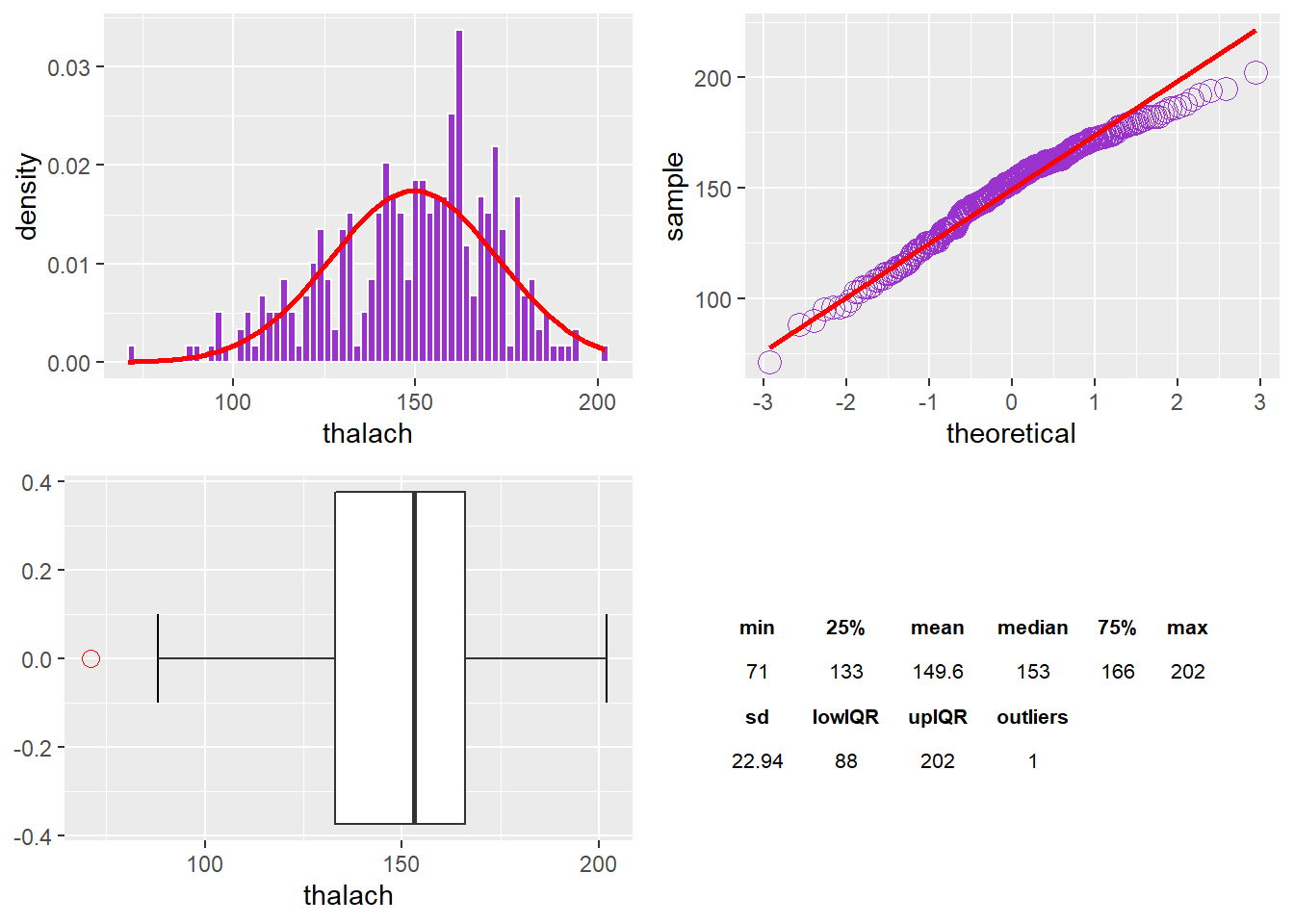
| thalach | 8 | 297 | 149.60 | 22.94 | 153.0 | 150.91 | 22.24 | 71 | 202.0 | 131.0 | -0.53 | -0.09 | 1.33 | 133 | 166.0 |
| exang | 9 | 297 | 0.33 | 0.47 | 0.0 | 0.28 | 0.00 | 0 | 1.0 | 1.0 | 0.74 | -1.46 | 0.03 | 0 | 1.0 |
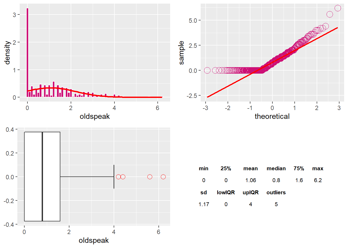
| oldspeak | 10 | 297 | 1.06 | 1.17 | 0.8 | 0.88 | 1.19 | 0 | 6.2 | 6.2 | 1.23 | 1.44 | 0.07 | 0 | 1.6 |
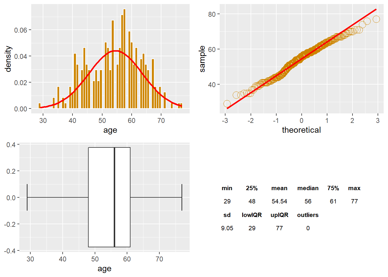
Numeric Variables Summary Plots - Histogram, Q-Q Plot, Boxplot, Summary Table
These next series of plots give a good visual understanding of the above statistics in Table 1.
The age Variable
The points show a broader peak (obtuse) with narrow tails and a negative kurtosis close to a normal distribution.
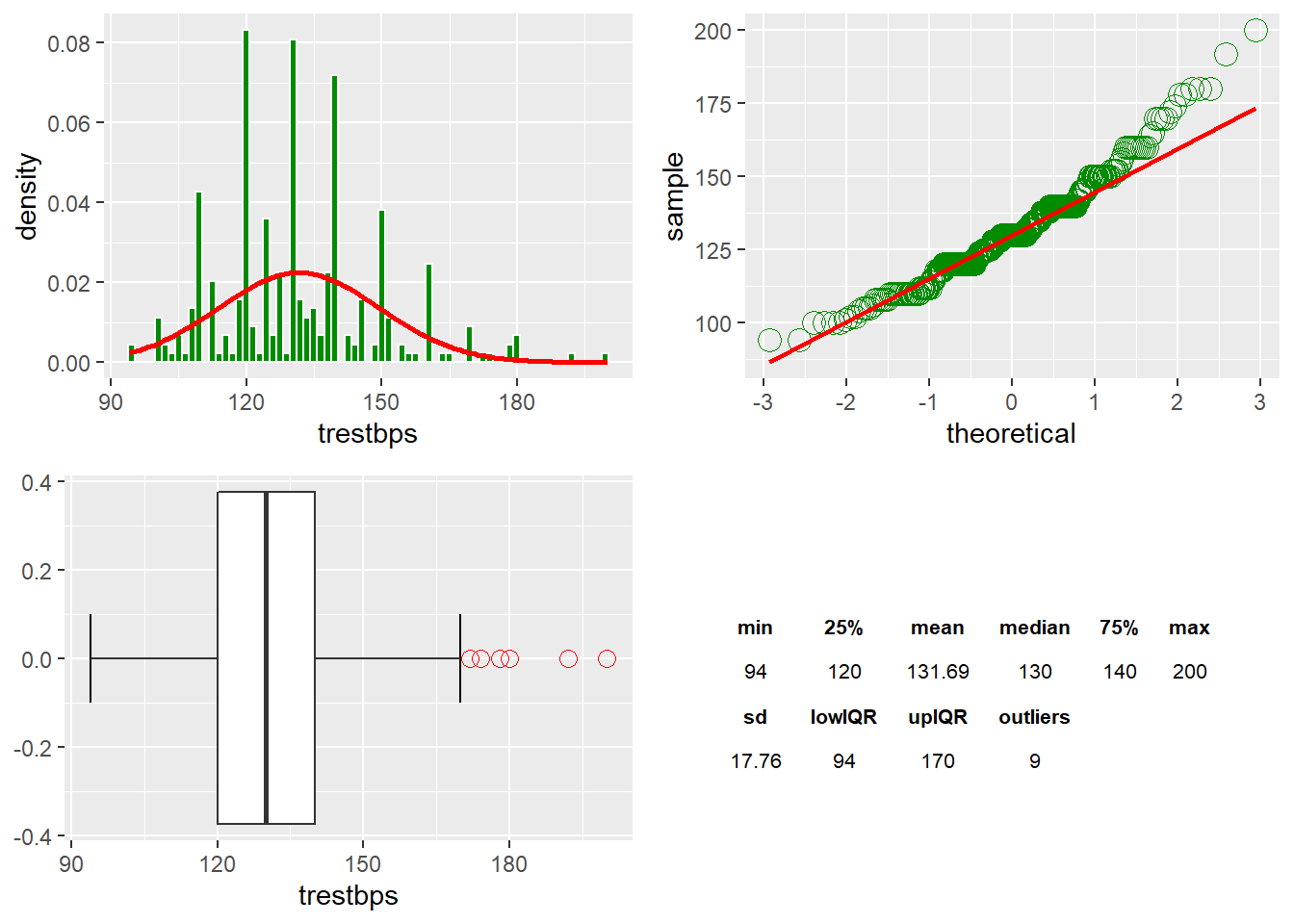
The trestbps Variable
There are nine outliers found in trestbps. I am noting the positive skew (right).
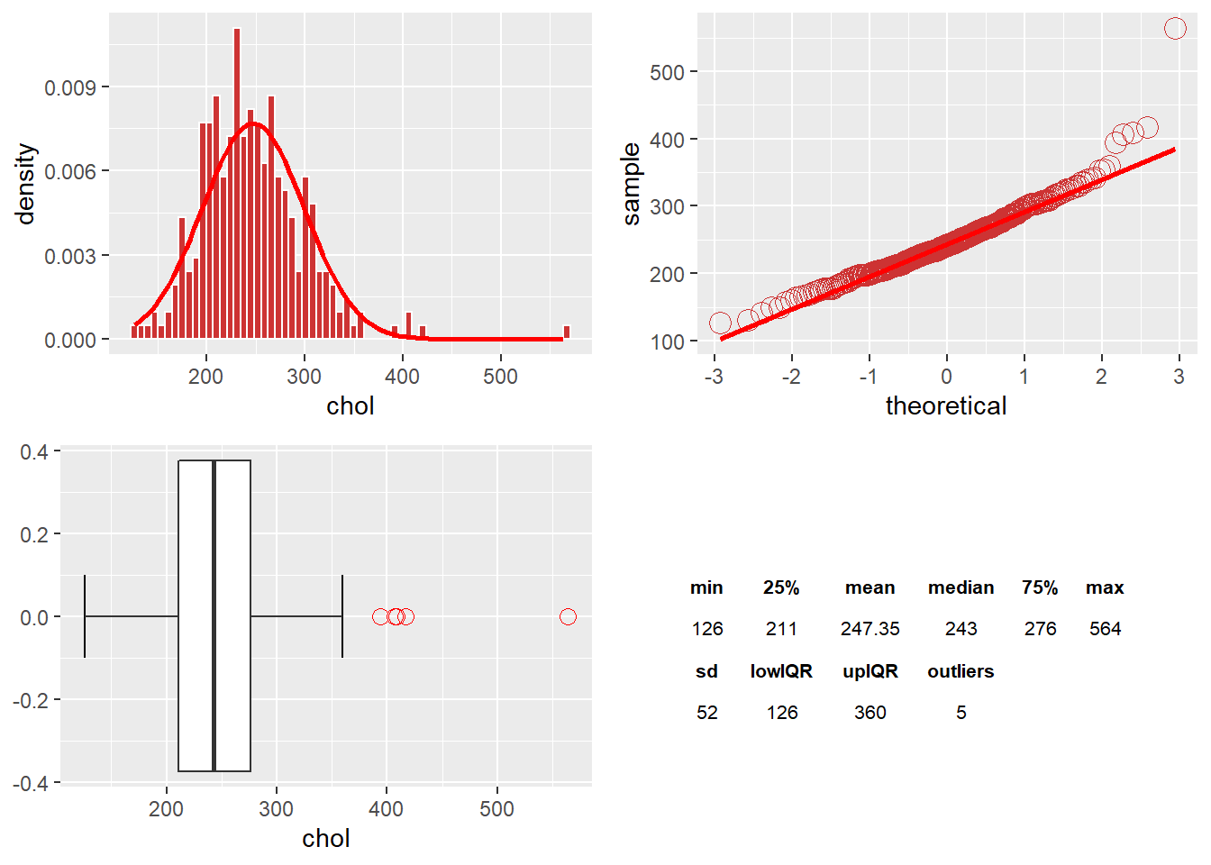
The chol Variable
There are five outliers in chol, which skews to the right. Removing the outliers will help
The thalach Variable
There is one outlier in thalach. I am observing a left or negative skew.
The oldspeak Variable
The variable oldspeak has five outliers and is right-skewed.
Outliers
Table 2 summarizes all of the outliers taken from the boxplot statistics above. The outlier is any value above the 75% quartile and below the 25% quartile. KNN is sensitive to these values per distance from the IQR.
| Value | Freq |
|---|---|
| 4.2 | 2 |
| 4.4 | 1 |
| 5.6 | 1 |
| 6.2 | 1 |
| 71 | 1 |
| 172 | 1 |
| 174 | 1 |
| 178 | 2 |
| 180 | 3 |
| 192 | 1 |
| 200 | 1 |
| 394 | 1 |
| 407 | 1 |
| 409 | 1 |
| 417 | 1 |
| 564 | 1 |
Remove Outliers
outL = filter(HD, trestbps >= 172 | chol >= 394 | thalach == 71 | oldspeak >= 4.2)
HD = HD %>% anti_join(outL)
Scale the Five Numeric Variables
rescaledata <- function(x) {
  return ((x - min(x)) / (max(x) - min(x)))
  }
HD = HD %>% mutate_at(c("age", "trestbps", "chol", "thalach", "oldspeak"), rescaledata)Rescaling Summary
## Rows: 278
## Columns: 14
## $ age      <dbl> 0.7083333, 0.7916667, 0.7916667, 0.1666667, 0.2500000, 0.5...
## $ sex      <dbl> 1, 1, 1, 1, 0, 1, 0, 0, 1, 1, 1, 0, 1, 1, 1, 1, 1, 0, 1, 1...
## $ cp       <fct> 1, 4, 4, 3, 2, 2, 4, 4, 4, 4, 4, 2, 3, 2, 3, 2, 4, 3, 2, 1...
## $ trestbps <dbl> 0.6710526, 0.8684211, 0.3421053, 0.4736842, 0.4736842, 0.3...
## $ chol     <dbl> 0.4572650, 0.6837607, 0.4401709, 0.5299145, 0.3333333, 0.4...
## $ fbs      <dbl> 1, 0, 0, 0, 0, 0, 0, 0, 0, 1, 0, 0, 1, 0, 0, 0, 0, 0, 0, 0...
## $ restecg  <fct> 2, 2, 2, 0, 2, 0, 2, 0, 2, 2, 0, 2, 2, 0, 0, 0, 0, 0, 0, 2...
## $ thalach  <dbl> 0.5438596, 0.1754386, 0.3596491, 0.8684211, 0.7368421, 0.7...
## $ exang    <dbl> 0, 1, 1, 0, 0, 0, 0, 1, 0, 1, 0, 0, 1, 0, 0, 0, 0, 0, 0, 1...
## $ oldspeak <dbl> 0.575, 0.375, 0.650, 0.875, 0.350, 0.200, 0.900, 0.150, 0....
## $ slope    <fct> 3, 2, 2, 3, 1, 1, 3, 1, 2, 3, 2, 2, 2, 1, 1, 3, 1, 1, 1, 2...
## $ ca       <fct> 0, 3, 2, 0, 0, 0, 2, 0, 1, 0, 0, 0, 1, 0, 0, 0, 0, 0, 0, 0...
## $ thal     <fct> 6, 3, 7, 3, 3, 3, 3, 3, 7, 7, 6, 3, 6, 7, 3, 7, 3, 3, 3, 3...
## $ num      <fct> No, Yes, Yes, No, No, No, Yes, No, Yes, Yes, No, No, Yes, ...
Re-encode Categorical Variables
Below is the code for creating new data columns from the categorical variables with classes more than two. I leave the variables with two classes or binary 0 & 1 because collinearity could happen if I broke them out into their columns. Thus they don’t need to be one-hot-encoded into dummy variables. sex, fbs, exang are binary, and the remaining are encoded.
HDn = bind_cols(HD,
  (as_tibble(
    predict(dummyVars(~ cp+restecg+slope+ca+thal,
                data = HD,
                levelsOnly = FALSE,
                sep = "_"),
      newdata = HD)))
)
Remove variables that the dummy variables replaced.
HD = select(HDn, -c(cp, restecg, slope, ca, thal, restecg_1))Data Summary after Cleaning
## Rows: 278
## Columns: 25
## $ age       <dbl> 0.7083333, 0.7916667, 0.7916667, 0.1666667, 0.2500000, 0....
## $ sex       <dbl> 1, 1, 1, 1, 0, 1, 0, 0, 1, 1, 1, 0, 1, 1, 1, 1, 1, 0, 1, ...
## $ trestbps  <dbl> 0.6710526, 0.8684211, 0.3421053, 0.4736842, 0.4736842, 0....
## $ chol      <dbl> 0.4572650, 0.6837607, 0.4401709, 0.5299145, 0.3333333, 0....
## $ fbs       <dbl> 1, 0, 0, 0, 0, 0, 0, 0, 0, 1, 0, 0, 1, 0, 0, 0, 0, 0, 0, ...
## $ thalach   <dbl> 0.5438596, 0.1754386, 0.3596491, 0.8684211, 0.7368421, 0....
## $ exang     <dbl> 0, 1, 1, 0, 0, 0, 0, 1, 0, 1, 0, 0, 1, 0, 0, 0, 0, 0, 0, ...
## $ oldspeak  <dbl> 0.575, 0.375, 0.650, 0.875, 0.350, 0.200, 0.900, 0.150, 0...
## $ num       <fct> No, Yes, Yes, No, No, No, Yes, No, Yes, Yes, No, No, Yes,...
## $ cp_1      <dbl> 1, 0, 0, 0, 0, 0, 0, 0, 0, 0, 0, 0, 0, 0, 0, 0, 0, 0, 0, ...
## $ cp_2      <dbl> 0, 0, 0, 0, 1, 1, 0, 0, 0, 0, 0, 1, 0, 1, 0, 1, 0, 0, 1, ...
## $ cp_3      <dbl> 0, 0, 0, 1, 0, 0, 0, 0, 0, 0, 0, 0, 1, 0, 1, 0, 0, 1, 0, ...
## $ cp_4      <dbl> 0, 1, 1, 0, 0, 0, 1, 1, 1, 1, 1, 0, 0, 0, 0, 0, 1, 0, 0, ...
## $ restecg_0 <dbl> 0, 0, 0, 1, 0, 1, 0, 1, 0, 0, 1, 0, 0, 1, 1, 1, 1, 1, 1, ...
## $ restecg_2 <dbl> 1, 1, 1, 0, 1, 0, 1, 0, 1, 1, 0, 1, 1, 0, 0, 0, 0, 0, 0, ...
## $ slope_1   <dbl> 0, 0, 0, 0, 1, 1, 0, 1, 0, 0, 0, 0, 0, 1, 1, 0, 1, 1, 1, ...
## $ slope_2   <dbl> 0, 1, 1, 0, 0, 0, 0, 0, 1, 0, 1, 1, 1, 0, 0, 0, 0, 0, 0, ...
## $ slope_3   <dbl> 1, 0, 0, 1, 0, 0, 1, 0, 0, 1, 0, 0, 0, 0, 0, 1, 0, 0, 0, ...
## $ ca_0      <dbl> 1, 0, 0, 1, 1, 1, 0, 1, 0, 1, 1, 1, 0, 1, 1, 1, 1, 1, 1, ...
## $ ca_1      <dbl> 0, 0, 0, 0, 0, 0, 0, 0, 1, 0, 0, 0, 1, 0, 0, 0, 0, 0, 0, ...
## $ ca_2      <dbl> 0, 0, 1, 0, 0, 0, 1, 0, 0, 0, 0, 0, 0, 0, 0, 0, 0, 0, 0, ...
## $ ca_3      <dbl> 0, 1, 0, 0, 0, 0, 0, 0, 0, 0, 0, 0, 0, 0, 0, 0, 0, 0, 0, ...
## $ thal_3    <dbl> 0, 1, 0, 1, 1, 1, 1, 1, 0, 0, 0, 1, 0, 0, 1, 0, 1, 1, 1, ...
## $ thal_6    <dbl> 1, 0, 0, 0, 0, 0, 0, 0, 0, 0, 1, 0, 1, 0, 0, 0, 0, 0, 0, ...
## $ thal_7    <dbl> 0, 0, 1, 0, 0, 0, 0, 0, 1, 1, 0, 0, 0, 1, 0, 1, 0, 0, 0, ...
Data Splitting
To create proportionate random splits of the data, I use the function createDataPartition. If the y argument to this function is a factor, random sampling occurs within each class. It preserves the overall class distribution of the data (stratified random sampling in the classes). Here I create the training data and testing data for the KNN classifier. I pick an arbitrary 70%/30% training/testing data split. Training is to build the KNN model, and the testing is to qualify the model performance.
set.seed(1254)
HD_Index <- createDataPartition(HD$num, p=0.7, list = FALSE, times = 1)
HD_train <- HD[HD_Index, ]
HD_test <- HD[-HD_Index, ]
Training and Test Data Split
## [1] 195## [1] 83k-Nearest Neighbor Using the Caret Library
The optimal starting value for k is the square root of the training data. The value is rounded to an odd value. Thus we should see significant improvements after k = 15, but will run this from k=1 for demonstration.
sqrt(nrow(HD_train))## [1] 13.96424k-Fold Cross-Validataion
The resampling method of repeated tenfold cross-fold, ten times (3 is normal), is repeated multiple times, results aggregated, and 100 hold-out sets used to estimate the model efficacy. The model will do class probability on binary or two class predictors and indicated by the last two arguments in trainControl below. The twoClassSummary argument computes the area under the ROC curve and the specificity and sensitivity under the 50% cutoff.
ctrl <- trainControl(method='repeatedcv',
                    number=10,
                    repeats=10,
                    classProbs = TRUE,
                    summaryFunction = twoClassSummary
                    )
Tuning Parameters
See below for the basic syntax for fitting this model using repeated cross-validation. Here I set the parameters using resampling and performance measures.
The first two arguments to the train function are the predictor and outcome data objects. The third argument, method = KNN, specifies the KNN algorithm. The fourth is the summary metric; we will evaluate the model for the receiver operator characteristic curve (ROC), and that will also give us the area under the curve (AUC). The data is pre-processed by centering (I scaled the data earlier, or do it here in this argument). The train function can automatically create a grid of tuning parameters. Also, I can specify the tuneGrid below. k starting at one and increasing by four up until 21, then increases by 20 up to 101 (odd k values only). Thus k == 1, 3, 5, 9, 13, 17, 21, 41, 61, 81, 101. I tried higher k but the ROC diminished.
set.seed(23)
KNNFit = train(num ~ .,
               data = HD_train,
               method = "knn",
               metric = "ROC",
               preProc = c("center"),
               tuneGrid = data.frame(.k = c(4*(0:5)+1,
                                            20*(1:5)+1)),
               trControl = ctrl)
Summary of the Training
Optimal k is 81. ROC of 92.2%, Sensitivity of 92.8% and Specificity of 73.6%
## k-Nearest Neighbors
##
## 195 samples
## 24 predictor
## 2 classes: 'No', 'Yes'
##
## Pre-processing: centered (24)
## Resampling: Cross-Validated (10 fold, repeated 10 times)
## Summary of sample sizes: 175, 175, 176, 176, 175, 177, ...
## Resampling results across tuning parameters:
##
## k ROC Sens Spec
## 1 0.7312942 0.7727273 0.6898611
## 5 0.8486572 0.8401818 0.7302778
## 9 0.8832936 0.8765455 0.7397222
## 13 0.8896749 0.8625455 0.7498611
## 17 0.8936199 0.8790909 0.7591667
## 21 0.8964564 0.8958182 0.7704167
## 41 0.9150537 0.9190000 0.7465278
## 61 0.9199495 0.9087273 0.7372222
## 81 0.9224066 0.9289091 0.7362500
## 101 0.9184438 0.9460000 0.7195833
##
## ROC was used to select the optimal model using the largest value.
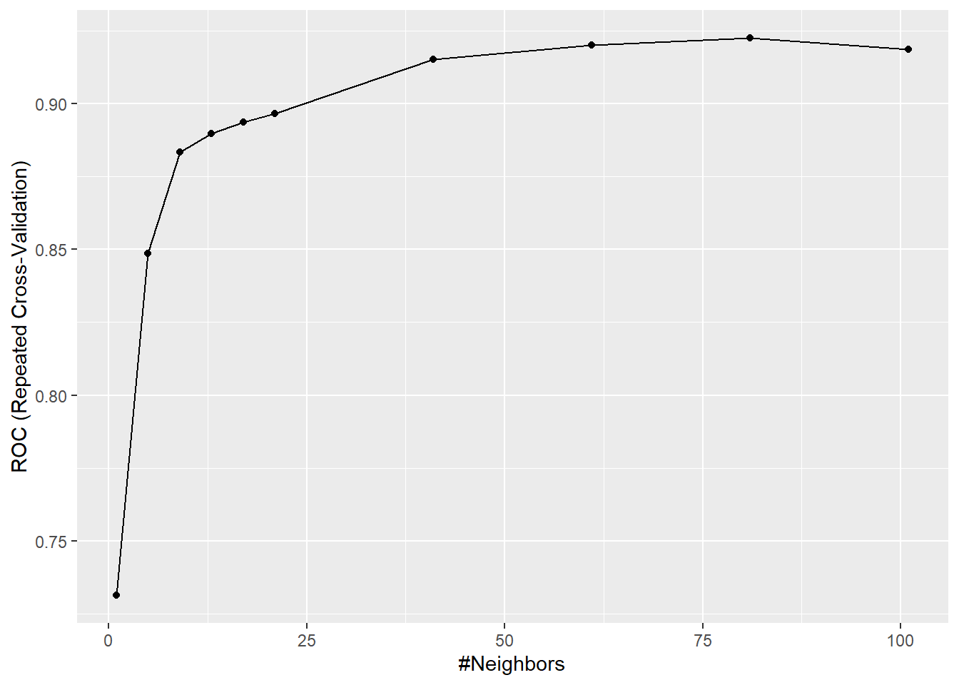
## The final value used for the model was k = 81.Plot of k increment up to k = 101
Run the Optimal Model on Test Data - Shows Probabilities
kpred = predict(KNNFit, newdata = HD_test, type= "prob")## No Yes
## 1 0.3580247 0.6419753
## 2 0.8888889 0.1111111
## 3 0.8024691 0.1975309
## 4 0.8888889 0.1111111
## 5 0.8765432 0.1234568
## 6 0.8271605 0.1728395Merge the k parameters with the predicted values.
KNNFit$pred = merge(KNNFit$pred, KNNFit$bestTune)Summary Table
The sensitivity is the rate of prediction that “No” is correct (true positive rate), and specificity is the rate of prediction of the “Yes” is correct (false positive rate). This problem is challenging because of the potential cost of life, such as heart disease going undetected by the algorithm (false negative) or making a false positive prediction of heart disease when the subject is not at risk. The receiver operating character curve (ROC) will summarize the two metrics. For data with two classes, there are specialized functions for measuring model performance.
We are looking for the best ROC value and will be a balance between sensitivity and specificity. The higher sensitivity means the model predicts the potential of the subject having heart disease a higher percentage of the actual cases with heart disease. At the same time, the specificity predicts the non-heart disease samples more accurately. In Table 3, k == 81 is optimal with a ROC of 92.2 and a sensitivity of 92.9%, and specificity of 73.6%. Meaning subjects without the disease may be diagnosed with it if we use this model. However, the model catches a large percentage of cases that have the disease.
| k | ROC | Sens | Spec | ROCSD | SensSD | SpecSD |
|---|---|---|---|---|---|---|
| 1 | 0.731 | 0.773 | 0.690 | 0.097 | 0.125 | 0.154 |
| 5 | 0.849 | 0.840 | 0.730 | 0.087 | 0.111 | 0.155 |
| 9 | 0.883 | 0.877 | 0.740 | 0.074 | 0.086 | 0.154 |
| 13 | 0.890 | 0.863 | 0.750 | 0.072 | 0.097 | 0.143 |
| 17 | 0.894 | 0.879 | 0.759 | 0.069 | 0.093 | 0.140 |
| 21 | 0.896 | 0.896 | 0.770 | 0.072 | 0.089 | 0.140 |
| 41 | 0.915 | 0.919 | 0.747 | 0.062 | 0.079 | 0.140 |
| 61 | 0.920 | 0.909 | 0.737 | 0.062 | 0.088 | 0.149 |
| 81 | 0.922 | 0.929 | 0.736 | 0.060 | 0.082 | 0.156 |
| 101 | 0.918 | 0.946 | 0.720 | 0.063 | 0.069 | 0.164 |
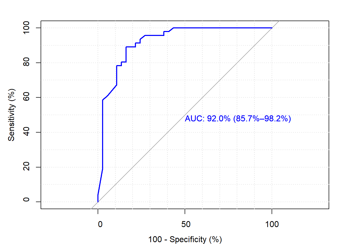
Receiver Operator Curve
KNNROC = roc(response = HD_test$num,
             predictor = kpred$Yes,
             levels = rev(levels(HD_test$num)),
               auc = TRUE,
               quiet = TRUE,
               grid=TRUE,
               percent = TRUE,
               ci = TRUE
               )
ROC Plot
The ROC gives the range of possible classification performances. The below graph is the ROC plot of Table 3. This model has a good time predicting the “No” or no presence of heart disease (92.9%); however, it struggles to predict the “Yes” for heart disease (Specificity = 73.6%). Lower specificity possibly attributed to the class imbalances we saw above in the categorical variables.
Confusion Matrix
The other method of evaluating the model fit is the confusion matrix and describes the k= 81 model predicted to actual classes. The metrics are True Positive, True Negative, False Positive, and False Negative. Accuracy is a product of the four results. The model’s accuracy predicted 44 “No” values correctly and 27 “Yes” Values correctly. The overall accuracy is 85.5% with a Kappa of 70.1%. Kappa does show moderate agreement between the actual and predicted classes; however, these metrics don’t distinguish the type of errors made or the frequencies of each class. Hence the ROC was a more appropriate measure for this exercise.
## Confusion Matrix and Statistics
##
##           Reference
## Prediction No Yes
##        No  44  10
##        Yes  2  27
##
##                Accuracy : 0.8554
##                  95% CI : (0.7611, 0.923)
##     No Information Rate : 0.5542
##     P-Value [Acc > NIR] : 4.732e-09
##
##                   Kappa : 0.7011
##
##  Mcnemar's Test P-Value : 0.04331
##
##             Sensitivity : 0.9565
##             Specificity : 0.7297
##          Pos Pred Value : 0.8148
##          Neg Pred Value : 0.9310
##              Prevalence : 0.5542
##          Detection Rate : 0.5301
##    Detection Prevalence : 0.6506
##       Balanced Accuracy : 0.8431
##
##        'Positive' Class : No
##
References
Bali, R., Sarkar, D. (2016). R Machine Learning by Example. Packt Publishing. (Chapter 2: KNN). ISBN-10:1784390844
James, G., Witten, D., Hastie, T., and Tibshirabi, R. (2013). An Introduction to Statistical Learning with Applications in R. DOI: 10.1007/978-1-4614-7138-7
Johnson, K., Kuhn, M. (2013). Applied Predictive Modeling. Springer-Verlag, DOI: 10.1007/978-1-4614-6849-3
MIT OpenCourseWare (2014). 10. Introduction to Learning, Nearest Neighbors. Retrieved from: https://www.youtube.com/watch?v=09mb78oiPkA
Saxena, A. (2011). Supervised Learning (CS5350/6350) - KNN. Cornell University. Retrieved from: http://www.cs.cornell.edu/courses/CS4758/2013sp/materials/cs4758-KNN-lectureslides.pdf