Naive Bayes SMS Message Classifier
This analysis demonstrates the naive bayes classifier in determining the spam or ham status of 4837 SMS messages. The data set is retrieved from: http://archive.ics.uci.edu/ml/datasets/SMS+Spam+Collection. The data needs explicit cleaning to prepare it to run through a naive bayes classifier. A training and test set is created to train and validate the predictive ability ofy the model. There are summary plots of the words found in abundance in the data. The summary will show the model’s predictive accuracy and the simplicity of running the data. Crossfold validation method is used and the Accuracy and Kappa are the metrics to judge performance.
Load Libraries
library(tidyverse)
library(e1071)
library(tm)
library(SnowballC)
library(wordcloud)
library(gmodels)
library(caret)
Download the Dataset
# place data into frame
url = "https://archive.ics.uci.edu/ml/machine-learning-databases/00228/smsspamcollection.zip"
# create temp file for the zip file
zip_file = tempfile(fileext = ".zip")
# unzip data into temp location
download.file(url, zip_file, method = 'libcurl', mode = "wb")
# read data into a tibble and specify data type for each variable, see EPA data source

SMSSpamCollection = read_delim(zip_file, delim = "\t", col_names = c("type", "text"), col_types = "ff")
# remove spaces in variables and replace with underscore
#names(SMSSpamCollection) = gsub("\\s", "_", names(SMSSpamCollection))
unlink(zip_file)
msg <- SMSSpamCollection #save to data frameglimpse(msg) #check data## Rows: 4,837
## Columns: 2
## $ type <fct> ham, ham, spam, ham, ham, spam, ham, ham, spam, spam, ham, spa...
## $ text <fct> "Go until jurong point, crazy.. Available only in bugis n grea...table(msg$type) # 13.2% spam 86.8% ham##
## ham spam
## 4199 638The first part of this analysis uses a dataset size of 3184 and runs through to prediction and accuracy measurement of the model. It was unknown that the data set is 4837 observations. That section will follow last. Thus this will be treated as an exercise in smaller verses larger data sets and how the two compare in accuracy. It is assumed the data is random and the model should work.
msg_corpus <- VCorpus(VectorSource(msg$text)) #create source object and sent to frameprint(msg_corpus) #check to see if documents are now stored## <<VCorpus>>
## Metadata: corpus specific: 0, document level (indexed): 0
## Content: documents: 4837inspect(msg_corpus[1:2]) #check summary of first two messages. ## <<VCorpus>>
## Metadata: corpus specific: 0, document level (indexed): 0
## Content: documents: 2
##
## [[1]]
## <<PlainTextDocument>>
## Metadata: 7
## Content: chars: 111
##
## [[2]]
## <<PlainTextDocument>>
## Metadata: 7
## Content: chars: 29as.character(msg_corpus[[1]]) #view actual first message## [1] "Go until jurong point, crazy.. Available only in bugis n great world la e buffet... Cine there got amore wat..."lapply(msg_corpus[1:2], as.character) #view fisrt two messages## $`1`
## [1] "Go until jurong point, crazy.. Available only in bugis n great world la e buffet... Cine there got amore wat..."
##
## $`2`
## [1] "Ok lar... Joking wif u oni..."msg_clean <- tm_map(msg_corpus, content_transformer(tolower))#transform to all lowercase letters
as.character(msg_clean[[1]]) # check that it worked on first line## [1] "go until jurong point, crazy.. available only in bugis n great world la e buffet... cine there got amore wat..."msg_clean <- tm_map(msg_clean, removeNumbers) #removes numbers from data
msg_clean <- tm_map(msg_clean, removeWords, stopwords()) #removes filler words
msg_clean <- tm_map(msg_clean, removePunctuation) #removes punctuation but ... can merge unwanted strings error
#This function creates error in DocumentTermMatrix step
#replacePunctuation <- function(x) {
# gsub("[[:punct:]]+"," ", x)
#}
#msg_clean <- tm_map(msg_clean, replacePunctuation) #Error
#msg_clean <- tm_map(msg_clean, PlainTextDocument) #showing alternate may work without error
as.character(msg_clean[[1]]) # check that punctuation is removed. ## [1] "go jurong point crazy available bugis n great world la e buffet cine got amore wat"as.character(msg_clean[[14]]) #check line 14 before stemming## [1] " searching right words thank breather promise wont take help granted will fulfil promise wonderful blessing times"msg_clean <- tm_map(msg_clean, stemDocument) #remove suffix from words
as.character(msg_clean[[14]]) #confirm line 14 for removed suffix's## [1] "search right word thank breather promis wont take help grant will fulfil promis wonder bless time"msg_clean <- tm_map(msg_clean, stripWhitespace) #removes extra white spaces between words
as.character(msg_clean[[14]]) #confirm even spacing now## [1] "search right word thank breather promis wont take help grant will fulfil promis wonder bless time"msg_dtm <- DocumentTermMatrix(msg_clean) #had errors needed to change removePunctuation function abovemsg_dtm #check## <<DocumentTermMatrix (documents: 4837, terms: 6605)>>
## Non-/sparse entries: 40119/31908266
## Sparsity : 100%
## Maximal term length: 40
## Weighting : term frequency (tf)dtm <- TermDocumentMatrix(msg_clean)
m <- as.matrix(dtm)
v <- sort(rowSums(m), decreasing=TRUE)
d <- data.frame(word =names(v), freq=v)Displaying the top 15 words and the frequency they are occurring in the data. The words call, now, get, free all seem like good spam words. The graphic is a word cloud and also demonstrated the 10 most dominant words. The list is more precise in this aspect of identifying top words.
head(d,15)## word freq
## call call 658
## ham ham 629
## now now 483
## get get 451
## can can 405
## will will 391
## just just 369
## come come 301
## free free 278
## ltgt ltgt 276
## know know 272
## day day 260
## like like 259
## love love 255
## want want 245set.seed(1234)
wordcloud(words = d$word, freq = d$freq, min.freq = 10,
max.words=175, random.order=FALSE, rot.per=0.35,
colors=brewer.pal(8, "Dark2"))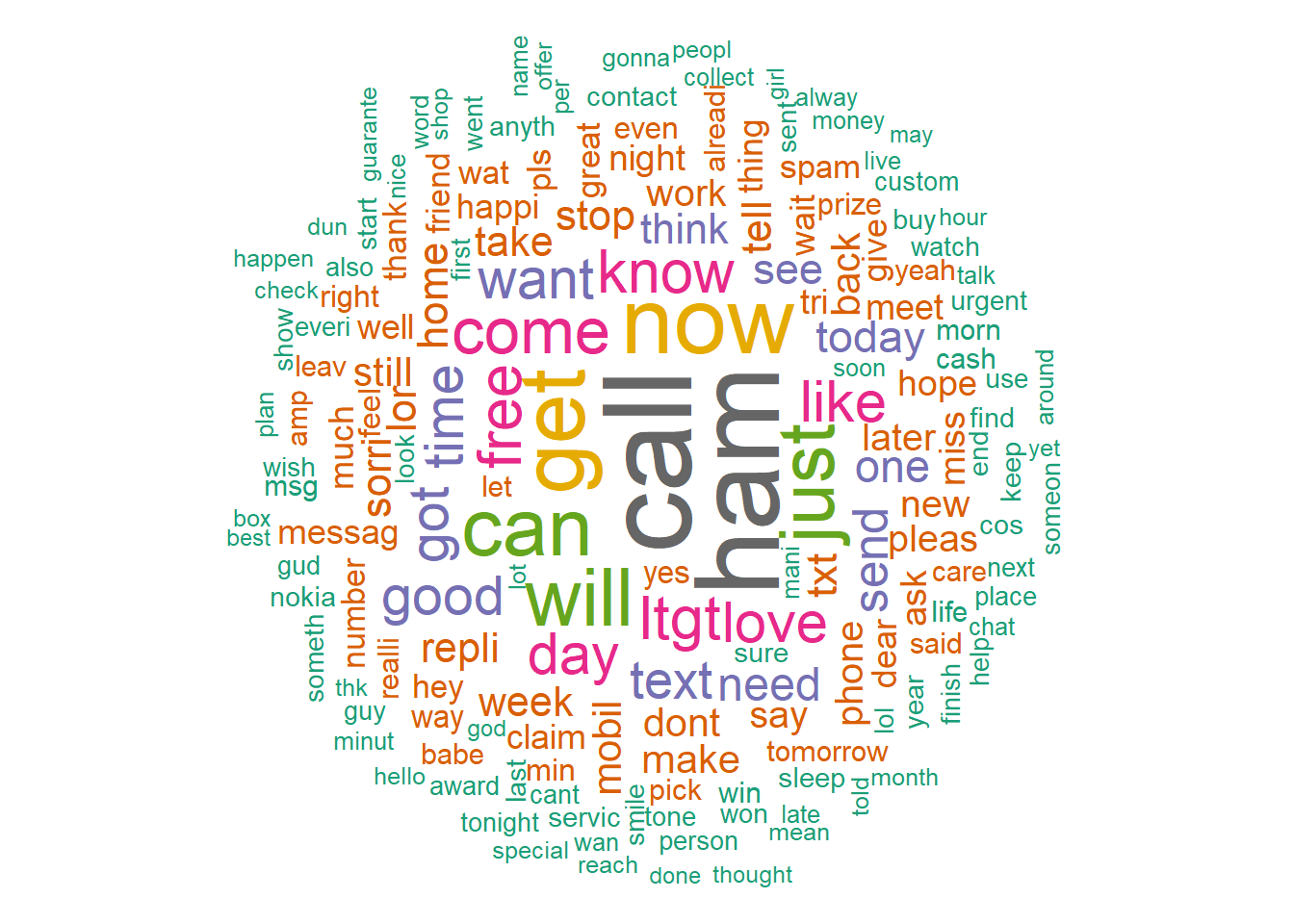
In the bar plot we get more of the same and another way to see the data. We can probably ignore the “ham” word and focus on the remaining words.
barplot(d[1:15,]$freq, las = 2, names.arg = d[1:15,]$word,
        col ="cornflowerblue", main ="15 Most Frequent Words",
        ylab = "Frequency")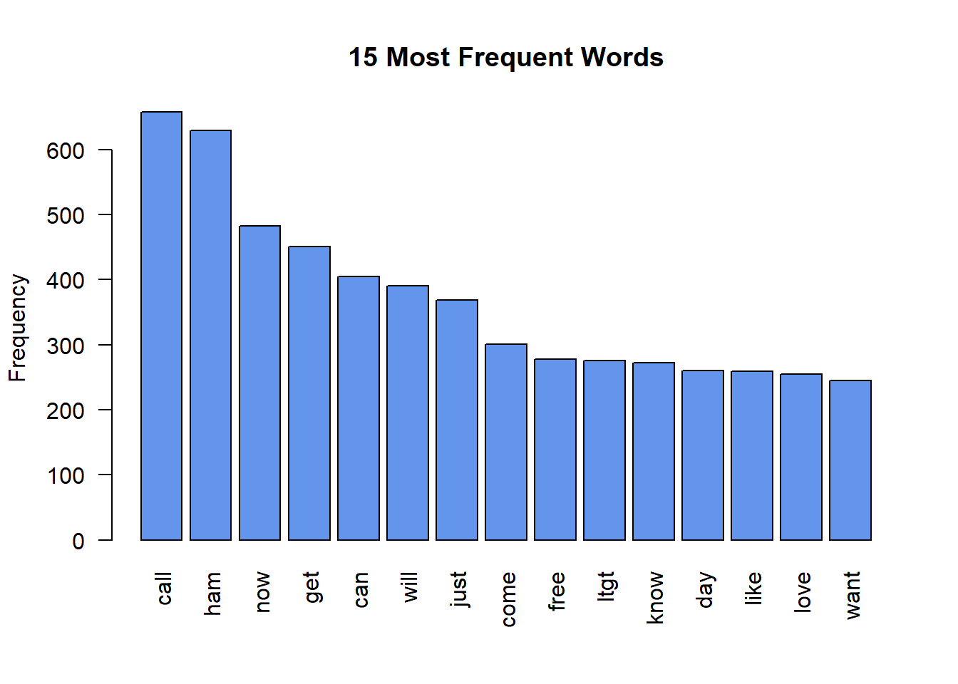
This word cloud doesn’t do much but show the dominant “ham” word. I doubt most will have the time to read through the text in this graphic.
ham <- subset(msg, type=="ham")wordcloud(ham$text, min.freq = 50, colors=brewer.pal(8, "Dark2"))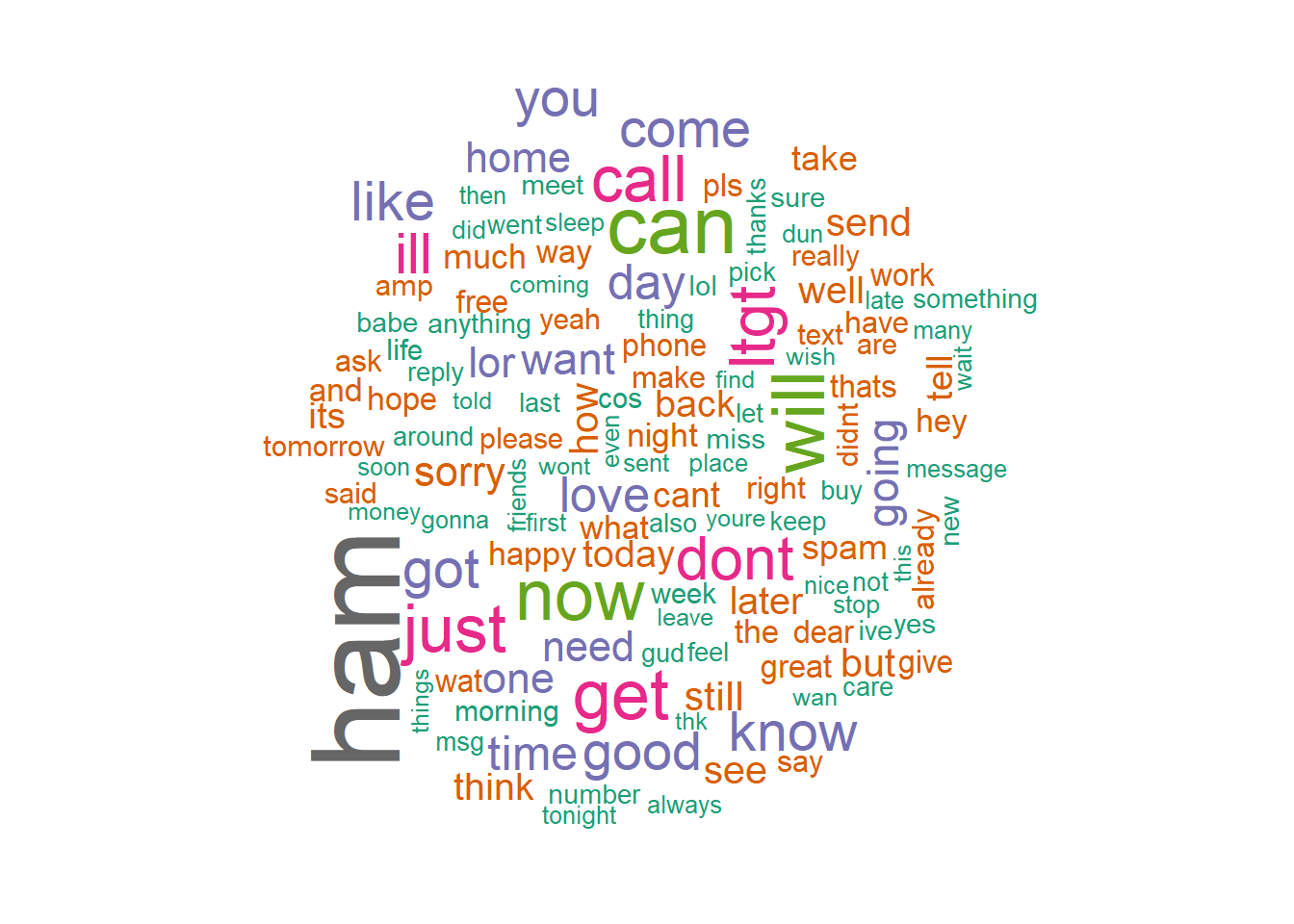
This graphic is more clear and again just displays what we already know from the simple table presented first. “call” “now” “free” sure standout as marketing terms.
spam <- subset(msg, type=="spam")wordcloud(spam$text, min.freq = 15, colors=brewer.pal(8, "Set1"))
Data Split - Training and Test Sets
msg_dtm_train <- msg_dtm[1:3385, ] #training set created
msg_dtm_test <- msg_dtm[3386:4837, ] #test set created

msg_train_labels <- msg[1:3385, ]$type #Create labels for table later
msg_test_labels <- msg[3386:4837, ]$type #create labels for table later
This is a check up on the proportions of train to test data and seems reasonable at 86% and 14%
#close to the first table 13% spam 87% ham.
prop.table(table(msg_train_labels)) #confirm labels are proportioned to train sets
## msg_train_labels
## ham spam
## 0.8691285 0.1308715#staying in close precentiles 87% and 13%
prop.table(table(msg_test_labels)) #confirm labels are proportioned to test sets## msg_test_labels
## ham spam
## 0.8657025 0.1342975Back to the overall text map. We still find top 10 near middle of graphic. At this point we get it and need to move on to the predictive model.
wordcloud(msg_clean, min.freq = 32, random.order = FALSE, colors=brewer.pal(8, "Set2"))#display 1% of the repetative words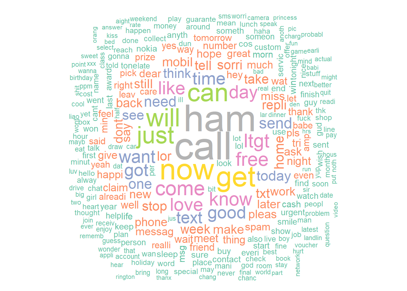
#wordcloud(msg_clean, min.freq = 32, random.order = FALSE, max.words = 5)
#wordcloud(msg$t, min.freq = 32, random.order = FALSE, max.words = 5)
msg_freq_words <- findFreqTerms(msg_dtm_train, 5) #get words that show at least 5 times, into frame
str(msg_freq_words) #check frame## chr [1:1086] "abiola" "abl" "abt" "accept" "access" "account" "across" ...msg_dtm_freq_train <- msg_dtm_train[ , msg_freq_words] #filter the DTM for the training set
msg_dtm_freq_test <- msg_dtm_test[ , msg_freq_words] #filter the DTM for the test set#change numeric 0,1 to character values for classifer to work
convert_counts <- function(x) {
x <- ifelse(x > 0, "yes", "no")
}msg_train <- apply(msg_dtm_freq_train, MARGIN = 2, convert_counts) #convert train set 0,1 to chars
msg_test <- apply(msg_dtm_freq_test, MARGIN = 2, convert_counts) #convert test set 0,1 to yes, nomsg_classifier <- naiveBayes(msg_train, msg_train_labels) #build the training model# 3385 total
msg_classifier$apriori## msg_train_labels
## ham spam
## 2942 443glimpse(msg_test)## chr [1:1452, 1:1086] "no" "no" "no" "no" "no" "no" "no" "no" "no" "no" ...
## - attr(*, "dimnames")=List of 2
## ..$ Docs : chr [1:1452] "3386" "3387" "3388" "3389" ...
## ..$ Terms: chr [1:1086] "abiola" "abl" "abt" "accept" ...glimpse(msg_train)## chr [1:3385, 1:1086] "no" "no" "no" "no" "no" "no" "no" "no" "no" "no" ...
## - attr(*, "dimnames")=List of 2
## ..$ Docs : chr [1:3385] "1" "2" "3" "4" ...
## ..$ Terms: chr [1:1086] "abiola" "abl" "abt" "accept" ...glimpse(msg_train_labels)## Factor w/ 2 levels "ham","spam": 1 1 2 1 1 2 1 1 2 2 ...set.seed(98)
msg_test_pred <- predict(msg_classifier, msg_test) #test the classifer on new dataHere is the predictive analysis. The table shows a total of 28 (2 + 26) were incorrectly classified and that is 2.9%. 2 out of 820 messages were misidentified as spam, while 26 of 135 messages were incorrectly labeled as ham. For a first try at Naive Bayes classification these results seem good granted the data is smaller than the 5574 intended size. The accuracy of the model is 97% with a kappa of 0.87. 26 incorrectly identified is still a little high but 2 is not bad.
#Create table to compare perdictions to true values
CrossTable(msg_test_pred, msg_test_labels,
           prop.chisq = FALSE, prop.t = FALSE,
           dnn = c('predicted', 'actual'))
##
##
## Cell Contents
## |-------------------------|
## | N |
## | N / Row Total |
## | N / Col Total |
## |-------------------------|
##
##
## Total Observations in Table: 1452
##
##
## | actual
## predicted | ham | spam | Row Total |
## -------------|-----------|-----------|-----------|
## ham | 1251 | 25 | 1276 |
## | 0.980 | 0.020 | 0.879 |
## | 0.995 | 0.128 | |
## -------------|-----------|-----------|-----------|
## spam | 6 | 170 | 176 |
## | 0.034 | 0.966 | 0.121 |
## | 0.005 | 0.872 | |
## -------------|-----------|-----------|-----------|
## Column Total | 1257 | 195 | 1452 |
## | 0.866 | 0.134 | |
## -------------|-----------|-----------|-----------|
##
## confusionMatrix(msg_test_pred, msg_test_labels, positive = 'spam')## Confusion Matrix and Statistics
##
## Reference
## Prediction ham spam
## ham 1251 25
## spam 6 170
##
## Accuracy : 0.9787
## 95% CI : (0.9698, 0.9854)
## No Information Rate : 0.8657
## P-Value [Acc > NIR] : < 2.2e-16
##
## Kappa : 0.9042
##
## Mcnemar's Test P-Value : 0.001225
##
## Sensitivity : 0.8718
## Specificity : 0.9952
## Pos Pred Value : 0.9659
## Neg Pred Value : 0.9804
## Prevalence : 0.1343
## Detection Rate : 0.1171
## Detection Prevalence : 0.1212
## Balanced Accuracy : 0.9335
##
## 'Positive' Class : spam
## Here we add laplace 1 to the model to see if we can improve accuracy. Instead we increase our incorrectly classified variables by 4 and 1 (6 and 27) and our accuracy and kappa drops 96.5% and 0.84. Still pretty high but not perfect.
msg_classifier2 <- naiveBayes(msg_train, msg_train_labels, laplace = 1) #adjust laplace to 1
msg_test_pred2 <- predict(msg_classifier2, msg_test)
CrossTable(msg_test_pred2, msg_test_labels,
prop.chisq = FALSE, prop.t = FALSE, prop.r = FALSE,
dnn = c('predicted', 'actual'))##
##
## Cell Contents
## |-------------------------|
## | N |
## | N / Col Total |
## |-------------------------|
##
##
## Total Observations in Table: 1452
##
##
## | actual
## predicted | ham | spam | Row Total |
## -------------|-----------|-----------|-----------|
## ham | 1251 | 31 | 1282 |
## | 0.995 | 0.159 | |
## -------------|-----------|-----------|-----------|
## spam | 6 | 164 | 170 |
## | 0.005 | 0.841 | |
## -------------|-----------|-----------|-----------|
## Column Total | 1257 | 195 | 1452 |
## | 0.866 | 0.134 | |
## -------------|-----------|-----------|-----------|
##
## confusionMatrix(msg_test_pred2, msg_test_labels, positive = 'spam')## Confusion Matrix and Statistics
##
## Reference
## Prediction ham spam
## ham 1251 31
## spam 6 164
##
## Accuracy : 0.9745
## 95% CI : (0.965, 0.982)
## No Information Rate : 0.8657
## P-Value [Acc > NIR] : < 2.2e-16
##
## Kappa : 0.8841
##
## Mcnemar's Test P-Value : 7.961e-05
##
## Sensitivity : 0.8410
## Specificity : 0.9952
## Pos Pred Value : 0.9647
## Neg Pred Value : 0.9758
## Prevalence : 0.1343
## Detection Rate : 0.1129
## Detection Prevalence : 0.1171
## Balanced Accuracy : 0.9181
##
## 'Positive' Class : spam
## #the laplace=1 estimator predicitve model did not improve performance because we can see (6+27)=33 incorrectly classified
#messages increases slightly from the 26 earlier. Section 2 - Replay
Here we will redo the previous steps with more data, or correctly, the 5574 points in the data set that did not import the first time. We will focus on the differences and look for any improvements over less data (3184 verses 5574).
#Start all over again
spam_raw <- SMSSpamCollection
names(spam_raw) <- c("type", "text") #label V1 and V2.
## tibble [4,837 x 2] (S3: spec_tbl_df/tbl_df/tbl/data.frame)
## $ type: Factor w/ 2 levels "ham","spam": 1 1 2 1 1 2 1 1 2 2 ...
## $ text: Factor w/ 4522 levels "Go until jurong point, crazy.. Available only in bugis n great world la e buffet... Cine there got amore wat...",..: 1 2 3 4 5 6 7 8 9 10 ...
## - attr(*, "problems")= tibble [39 x 5] (S3: tbl_df/tbl/data.frame)
## ..$ row : int [1:39] 283 283 454 454 454 454 454 454 454 476 ...
## ..$ col : chr [1:39] "text" "text" "text" "text" ...
## ..$ expected: chr [1:39] "delimiter or quote" "delimiter or quote" "delimiter or quote" "delimiter or quote" ...
## ..$ actual : chr [1:39] " " "H" " " "Y" ...
## ..$ file : chr [1:39] "'C:\\Users\\Zeus\\AppData\\Local\\Temp\\RtmpOqCqTb\\fileca8340c50a2.zip'" "'C:\\Users\\Zeus\\AppData\\Local\\Temp\\RtmpOqCqTb\\fileca8340c50a2.zip'" "'C:\\Users\\Zeus\\AppData\\Local\\Temp\\RtmpOqCqTb\\fileca8340c50a2.zip'" "'C:\\Users\\Zeus\\AppData\\Local\\Temp\\RtmpOqCqTb\\fileca8340c50a2.zip'" ...
## - attr(*, "spec")=
## .. cols(
## .. type = col_factor(levels = NULL, ordered = FALSE, include_na = FALSE),
## .. text = col_factor(levels = NULL, ordered = FALSE, include_na = FALSE)
## .. )glimpse(msg2$type)## Factor w/ 2 levels "ham","spam": 1 1 2 1 1 2 1 1 2 2 ...msg_corpus2 <- VCorpus(VectorSource(msg2$text)) #create source object and sent to frame
msg_clean2 <- tm_map(msg_corpus2, content_transformer(tolower))#transform to all lowercase letters
msg_clean2 <- tm_map(msg_clean2, removeNumbers) #removes numbers from data
msg_clean2 <- tm_map(msg_clean2, removeWords, stopwords()) #removes filler words
msg_clean2 <- tm_map(msg_clean2, removePunctuation) #removes punctuation but ... can merge unwanted strings
msg_clean2 <- tm_map(msg_clean2, stemDocument) #remove suffix from words
msg_clean2 <- tm_map(msg_clean2, stripWhitespace) #removes extra white spaces between words
msg_dtm2 <- DocumentTermMatrix(msg_clean2)
dtm2 <- TermDocumentMatrix(msg_clean2)#top 10 words
m2 <- as.matrix(dtm2)
v2 <- sort(rowSums(m2), decreasing=TRUE)
d2 <- data.frame(word =names(v2), freq=v2)We can see “ham” and “spam” are out and “call”, “now”, “get”..“free” are still in the top words grouping.
head(d2,10)## word freq
## call call 658
## ham ham 629
## now now 483
## get get 451
## can can 405
## will will 391
## just just 369
## come come 301
## free free 278
## ltgt ltgt 276This graphic is working much better and the color coding is working to group similar frequent terms.
set.seed(4567)
wordcloud(words = d2$word, freq = d2$freq, min.freq = 1,
max.words=200, random.order=FALSE, rot.per=0.35,
colors=brewer.pal(8, "Dark2"))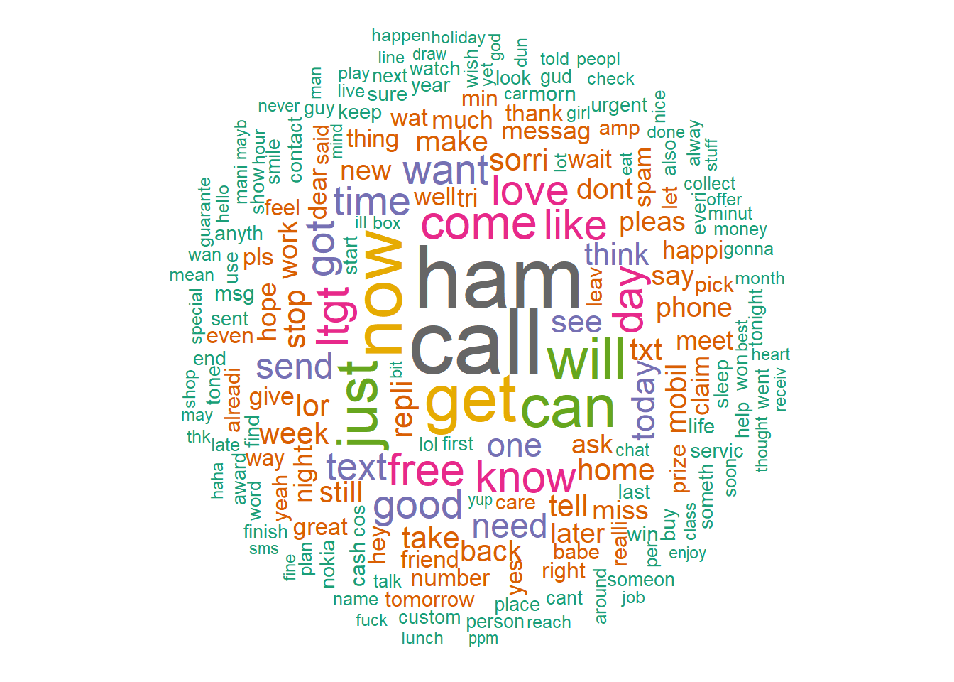 Oddly, “ham”/“spam” are back in the bar plot. But it is better than before because we can see the other words that dominate spam messaging.
barplot(d2[1:10,]$freq, las = 2, names.arg = d[1:10,]$word,
        col ="brown3", main ="Most frequent words",
        ylab = "Word frequencies")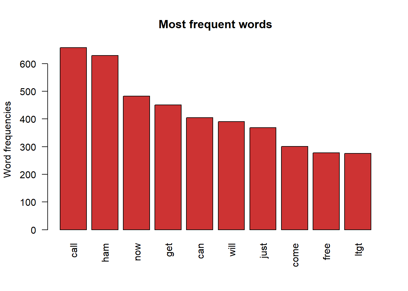
This graphic is producing some problems. The frequency was increased to 55 or 1% of the data size. And reduced the warning messages down to two from 10 prior before publishing these results. Interesting many messages have “sorry” in them or “need”….
ham2 <- subset(msg2, type=="ham")
wordcloud(ham2$text, min.freq = 55, colors=brewer.pal(8, "Dark2"))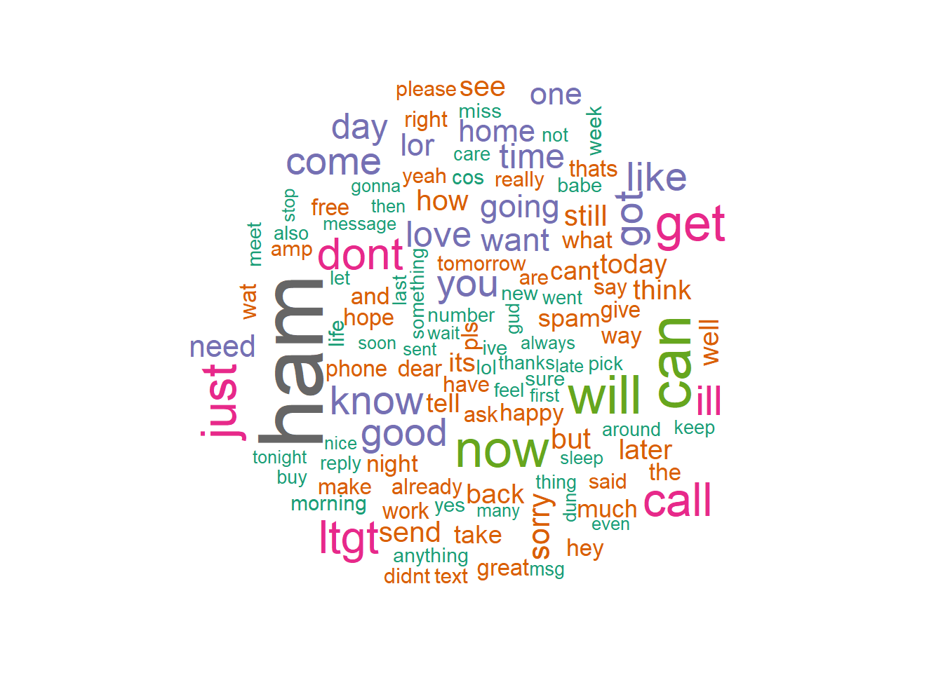
This graphic is better and definitely shows some of the spammy type words: get, mobile, prize, call, reply, stop, etc. Also increased the frequency to 55 from the first attempt at this.
spam2 <- subset(msg, type=="spam")
wordcloud(spam2$text, min.freq = 15, colors=brewer.pal(8, "Dark2"))
msg_dtm_train2 <- msg_dtm2[1:3385, ] #training set created
msg_dtm_test2 <- msg_dtm2[3386:4837, ] #test set created
msg_train_labels2 <- msg2[1:3385, ]$type #Create labels for table later
msg_test_labels2 <- msg2[3386:4837, ]$type #create labels for table laterThe proportions are the same as before because we used a calculator to figure a 70/30 split.
prop.table(table(msg_train_labels2)) #confirm labels are proportioned to train sets## msg_train_labels2
## ham spam
## 0.8691285 0.1308715prop.table(table(msg_test_labels2)) #confirm labels are proportioned to test sets## msg_test_labels2
## ham spam
## 0.8657025 0.1342975#wordcloud(msg_clean2, min.freq = 32, random.order = FALSE)#display 1% of the repetative words
#wordcloud(msg_clean2, min.freq = 32, random.order = FALSE, max.words = 5)msg_freq_words2 <- findFreqTerms(msg_dtm_train2, 5) #get words that show at least 5 times, into frame
msg_dtm_freq_train2 <- msg_dtm_train2[ , msg_freq_words2] #filter the DTM for the training set
msg_dtm_freq_test2 <- msg_dtm_test2[ , msg_freq_words2] #filter the DTM for the test set#change numeric 0,1 to character values for classifer to work
convert_counts2 <- function(x) {
x <- ifelse(x > 0, "yes", "no")
}msg_train2 <- apply(msg_dtm_freq_train2, MARGIN = 2, convert_counts2) #convert train set 0,1 to chars
msg_test2 <- apply(msg_dtm_freq_test2, MARGIN = 2, convert_counts2) #convert test set 0,1 to yes, no
msg_classifier2 <- naiveBayes(msg_train2, msg_train_labels2, laplace = 1) #build the training model and place in frame
msg_test_pred3 <- predict(msg_classifier2, msg_test2) #test the classifer on new data
#Create table to compare perdictions to true valuesThis time we show the laplace 1 first and show how it increases the incorrectly identified units of 5 + 33 to 38 higher than our first model of 2+26= 28. However, the accuracy climbs to 97.7% and a bigger kappa or 0.898. Improvements on accuracy and kappa but slightly more incorrectly labeled terms.
CrossTable(msg_test_pred3, msg_test_labels2,
           prop.chisq = FALSE, prop.t = FALSE,
           dnn = c('predicted', 'actual'))
##
##
## Cell Contents
## |-------------------------|
## | N |
## | N / Row Total |
## | N / Col Total |
## |-------------------------|
##
##
## Total Observations in Table: 1452
##
##
## | actual
## predicted | ham | spam | Row Total |
## -------------|-----------|-----------|-----------|
## ham | 1251 | 31 | 1282 |
## | 0.976 | 0.024 | 0.883 |
## | 0.995 | 0.159 | |
## -------------|-----------|-----------|-----------|
## spam | 6 | 164 | 170 |
## | 0.035 | 0.965 | 0.117 |
## | 0.005 | 0.841 | |
## -------------|-----------|-----------|-----------|
## Column Total | 1257 | 195 | 1452 |
## | 0.866 | 0.134 | |
## -------------|-----------|-----------|-----------|
##
## confusionMatrix(msg_test_pred3, msg_test_labels2, positive = 'spam')## Confusion Matrix and Statistics
##
## Reference
## Prediction ham spam
## ham 1251 31
## spam 6 164
##
## Accuracy : 0.9745
## 95% CI : (0.965, 0.982)
## No Information Rate : 0.8657
## P-Value [Acc > NIR] : < 2.2e-16
##
## Kappa : 0.8841
##
## Mcnemar's Test P-Value : 7.961e-05
##
## Sensitivity : 0.8410
## Specificity : 0.9952
## Pos Pred Value : 0.9647
## Neg Pred Value : 0.9758
## Prevalence : 0.1343
## Detection Rate : 0.1129
## Detection Prevalence : 0.1171
## Balanced Accuracy : 0.9181
##
## 'Positive' Class : spam
## # more accurate 98%, Kappa at 0.92msg_classifier4 <- naiveBayes(msg_train2, msg_train_labels2) #build the training model and place in frame
msg_test_pred4 <- predict(msg_classifier4, msg_test2) #test the classifer on new dataWhen the laplace 1 is dropped the model also drops the number of incorrectly labeled variables to 6+25= 31. This is still higher than the first model 2+26=28. But with it comes a higher accuracy of 98% and a higher kappa of 0.92! We show the highest accuracy and kappa of 4 trials using the larger data set (5574) however, the incorrectly labeled variables from the smaller data set produced lower mislabeling of 28 verse 31 in this model. So we can see a slight increase of one aspect and decrease in another. More model tuning should take place to refine this prediction to see where the error rate can be reduced.
CrossTable(msg_test_pred4, msg_test_labels2,
           prop.chisq = FALSE, prop.t = FALSE,
           dnn = c('predicted', 'actual'))
##
##
## Cell Contents
## |-------------------------|
## | N |
## | N / Row Total |
## | N / Col Total |
## |-------------------------|
##
##
## Total Observations in Table: 1452
##
##
## | actual
## predicted | ham | spam | Row Total |
## -------------|-----------|-----------|-----------|
## ham | 1251 | 25 | 1276 |
## | 0.980 | 0.020 | 0.879 |
## | 0.995 | 0.128 | |
## -------------|-----------|-----------|-----------|
## spam | 6 | 170 | 176 |
## | 0.034 | 0.966 | 0.121 |
## | 0.005 | 0.872 | |
## -------------|-----------|-----------|-----------|
## Column Total | 1257 | 195 | 1452 |
## | 0.866 | 0.134 | |
## -------------|-----------|-----------|-----------|
##
## confusionMatrix(msg_test_pred4, msg_test_labels2, positive = 'spam')## Confusion Matrix and Statistics
##
## Reference
## Prediction ham spam
## ham 1251 25
## spam 6 170
##
## Accuracy : 0.9787
## 95% CI : (0.9698, 0.9854)
## No Information Rate : 0.8657
## P-Value [Acc > NIR] : < 2.2e-16
##
## Kappa : 0.9042
##
## Mcnemar's Test P-Value : 0.001225
##
## Sensitivity : 0.8718
## Specificity : 0.9952
## Pos Pred Value : 0.9659
## Neg Pred Value : 0.9804
## Prevalence : 0.1343
## Detection Rate : 0.1171
## Detection Prevalence : 0.1212
## Balanced Accuracy : 0.9335
##
## 'Positive' Class : spam
##