Decision Tree and Random Forest
This analysis will utilize the data set from https://archive.ics.uci.edu/ml/machine-learning-databases/wine-quality/winequality-red.csv and the purpose is to find the differences between the decision tree method and the random forest method for predicting wine quality from the 11 variables that indicate each wine’s chemical readings. The 12th variable is the quality rating given to these 1599 wines and is used as the predictor in the models. The quality has ratings from 3 to 8. To make the ratings work in the models there will be three groups “Fair” = (3-4), “Satisfactory” = (5-6), and “Excellent” = (7-8).
# Load All Libraries
library(C50)
library(gmodels)
library(randomForest)
library(rpart)
library(rpart.plot)
library(caret)
#Load Data set
winequality.red <- read.csv("https://archive.ics.uci.edu/ml/machine-learning-databases/wine-quality/winequality-red.csv", row.names=NULL, sep=";")
vino1 <- winequality.redGlancing over the summary table we can see the quality is 3 to 8. The density is interesting because it is approximately 1. Maybe this is an important measure or maybe not, we will leave it in for now. The total.sulfur.dioxide is also interesting because it the max=289 while the mean=46.47 indicates some outlier values, but again lets keep the data to gather for now.
summary(vino1)## fixed.acidity volatile.acidity citric.acid residual.sugar
## Min. : 4.60 Min. :0.1200 Min. :0.000 Min. : 0.900
## 1st Qu.: 7.10 1st Qu.:0.3900 1st Qu.:0.090 1st Qu.: 1.900
## Median : 7.90 Median :0.5200 Median :0.260 Median : 2.200
## Mean : 8.32 Mean :0.5278 Mean :0.271 Mean : 2.539
## 3rd Qu.: 9.20 3rd Qu.:0.6400 3rd Qu.:0.420 3rd Qu.: 2.600
## Max. :15.90 Max. :1.5800 Max. :1.000 Max. :15.500
## chlorides free.sulfur.dioxide total.sulfur.dioxide density
## Min. :0.01200 Min. : 1.00 Min. : 6.00 Min. :0.9901
## 1st Qu.:0.07000 1st Qu.: 7.00 1st Qu.: 22.00 1st Qu.:0.9956
## Median :0.07900 Median :14.00 Median : 38.00 Median :0.9968
## Mean :0.08747 Mean :15.87 Mean : 46.47 Mean :0.9967
## 3rd Qu.:0.09000 3rd Qu.:21.00 3rd Qu.: 62.00 3rd Qu.:0.9978
## Max. :0.61100 Max. :72.00 Max. :289.00 Max. :1.0037
## pH sulphates alcohol quality
## Min. :2.740 Min. :0.3300 Min. : 8.40 Min. :3.000
## 1st Qu.:3.210 1st Qu.:0.5500 1st Qu.: 9.50 1st Qu.:5.000
## Median :3.310 Median :0.6200 Median :10.20 Median :6.000
## Mean :3.311 Mean :0.6581 Mean :10.42 Mean :5.636
## 3rd Qu.:3.400 3rd Qu.:0.7300 3rd Qu.:11.10 3rd Qu.:6.000
## Max. :4.010 Max. :2.0000 Max. :14.90 Max. :8.000Here the quality variable is grouped into categories because we can see in the barplot that there is a three way split in the quality ratings. Fair, Satisfactory, and Excellent will be used as the dependent variable. From the graph we can see the Satisfactory quality is about 82% of the data, Excellent is approximately 14% of the data and Fair is 0.4% of the data. In this example we have a good amount of data to indicate a normal quality wine in the middle. The Excellent wines are a metric that may be something we aim for if producing high quality wines. While the fair wines don’t have much data and possibly a good measure of what not to do when making a wine.
barplot(table(vino1$quality))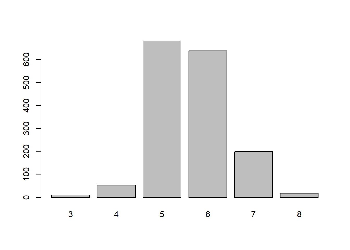
#group quality variable into 3
vino1$quality[vino1$quality >= 7] <- "Excellent"
vino1$quality[vino1$quality >= 5 & vino1$quality <=6] <- "Satisfactory"
vino1$quality[vino1$quality <= 4] <- "Fair"
#change quality to factor
vino1$quality <- as.factor(vino1$quality)
#view data set
str(vino1$quality)
## Factor w/ 3 levels "Excellent","Fair",..: 3 3 3 3 3 3 3 1 1 3 ...table(vino1$quality)##
## Excellent Fair Satisfactory
## 217 63 1319barplot(table(vino1$quality))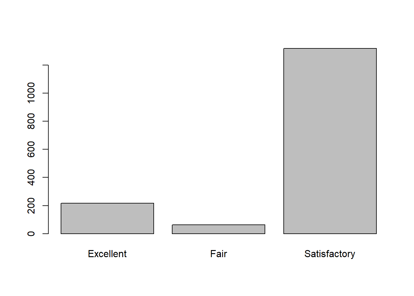
Part 1 - Decision Tree with C5.0 package
The first section is going to use the C5.0 package to model a decision tree. The data is split 70%/30% train/test for this project. The data is randomly sampled into training and test objects. In the training set we can see 83% Satisfactory, 13% Excellent, and 0.4% fair which are close to representing the data split mentioned earlier. The C5.0 model shows 1119 samples and the 11 predictors with a tree size of 54. The output is a bit lengthy and toward the end we can see the error at 5.8% which doesn’t seem too bad, but we will try to improve on later. The accuracy would be (106+21+927)/1119= 94% over the training data. The attributes usage is interesting and shows the top two attributes alcohol (100%) and volatile.acidity(96.25%). Then a sharp drop to sulfates at 34.5%. As mentioned earlier the density was about 1 and here we see its last for attributes at 2.32%. The attribute usage chart could possibly be used to limit variables in future decision trees by dropping the bottom four under 10%. For now we will proceed through the exercise with all the attributes to see what happens.
###############Decision Tree in C5.0
set.seed(1234)
train_sample <- sample(1599, 1119) #70/30 data split
str(train_sample) #check sample
## int [1:1119] 1308 1018 1125 1004 623 905 645 934 400 900 ...vino_train <- vino1[train_sample, ] #training set
vino_test <- vino1[-train_sample, ] #testing set
prop.table((table(vino_train$quality))) #Check split##
## Excellent Fair Satisfactory
## 0.13404826 0.04468275 0.82126899#library(C50)
set.seed(765)
vino_model <- C5.0(vino_train[-12], vino_train$quality) #training set less quality variablevino_model #check model##
## Call:
## C5.0.default(x = vino_train[-12], y = vino_train$quality)
##
## Classification Tree
## Number of samples: 1119
## Number of predictors: 11
##
## Tree size: 69
##
## Non-standard options: attempt to group attributesThis shows the predictive model and the cross table produces a summary. The model accuracy is 83% (40+1+359)/(480). The false positive of 34 and the false negative of 19 show there could be a fuzzy area between Excellent and Satisfactory. There is also a discrepancy between Fair and Satisfactory. With satisfactory being a large grouping there is room for error but it would be nice to have more accuracy on the higher end wines in the Excellent category.
vino_pred <- predict(vino_model, vino_test) #run prediction
#library(gmodels)
#Table outcome
CrossTable(vino_test$quality, vino_pred, prop.chisq = FALSE, prop.c = FALSE,
           prop.r = FALSE, dnn = c('actual quality', 'predicted quality'))
##
##
## Cell Contents
## |-------------------------|
## | N |
## | N / Table Total |
## |-------------------------|
##
##
## Total Observations in Table: 480
##
##
## | predicted quality
## actual quality | Excellent | Fair | Satisfactory | Row Total |
## ---------------|--------------|--------------|--------------|--------------|
## Excellent | 28 | 1 | 38 | 67 |
## | 0.058 | 0.002 | 0.079 | |
## ---------------|--------------|--------------|--------------|--------------|
## Fair | 1 | 1 | 11 | 13 |
## | 0.002 | 0.002 | 0.023 | |
## ---------------|--------------|--------------|--------------|--------------|
## Satisfactory | 28 | 15 | 357 | 400 |
## | 0.058 | 0.031 | 0.744 | |
## ---------------|--------------|--------------|--------------|--------------|
## Column Total | 57 | 17 | 406 | 480 |
## ---------------|--------------|--------------|--------------|--------------|
##
## confusionMatrix(vino_test$quality, vino_pred, dnn = c('actual quality', 'predicted quality'))## Confusion Matrix and Statistics
##
## predicted quality
## actual quality Excellent Fair Satisfactory
## Excellent 28 1 38
## Fair 1 1 11
## Satisfactory 28 15 357
##
## Overall Statistics
##
## Accuracy : 0.8042
## 95% CI : (0.7658, 0.8387)
## No Information Rate : 0.8458
## P-Value [Acc > NIR] : 0.9941
##
## Kappa : 0.2946
##
## Mcnemar's Test P-Value : 0.5458
##
## Statistics by Class:
##
## Class: Excellent Class: Fair Class: Satisfactory
## Sensitivity 0.49123 0.058824 0.8793
## Specificity 0.90780 0.974082 0.4189
## Pos Pred Value 0.41791 0.076923 0.8925
## Neg Pred Value 0.92978 0.965739 0.3875
## Prevalence 0.11875 0.035417 0.8458
## Detection Rate 0.05833 0.002083 0.7438
## Detection Prevalence 0.13958 0.027083 0.8333
## Balanced Accuracy 0.69951 0.516453 0.6491The next part of the C5.0 model is to try to improve the accuracy by increasing the number of trials to 10, which is the base point for most boosted models. The output is rather long. The Attribute usage is now showing 100% usage of alcohol, sulphates (from the first model) and includes density, total.sulfur.dioxide, and volatile.acidity. The remaining are in the 90% range with pH down to 86.6%. Thus with 10 trials more chances for the attributes to be utilized.The model classified 99% or a 0.71% error rate on the training data which is a big improvement from the 5.8% error we had earlier with one pass over the data. The accuracy only climbed up to 86% with 10 trials. A small gain but worth noting and looking further into possibly increasing the trials with more time for analysis. Not sure what to do to increase accuracy, the error rate over the training data is really low with the boost.
vino_boost <- C5.0(vino_train[-12], vino_train$quality, trials = 10) #try to improve
vino_boost
##
## Call:
## C5.0.default(x = vino_train[-12], y = vino_train$quality, trials = 10)
##
## Classification Tree
## Number of samples: 1119
## Number of predictors: 11
##
## Number of boosting iterations: 10
## Average tree size: 60.8
##
## Non-standard options: attempt to group attributesvino_boost$boostResults # long summary## Trial Size Errors Percent Data
## 1 1 69 52 4.6 Training Set
## 2 2 40 140 12.5 Training Set
## 3 3 59 145 13.0 Training Set
## 4 4 62 134 12.0 Training Set
## 5 5 70 110 9.8 Training Set
## 6 6 60 122 10.9 Training Set
## 7 7 68 105 9.4 Training Set
## 8 8 48 192 17.2 Training Set
## 9 9 77 133 11.9 Training Set
## 10 10 55 121 10.8 Training Setset.seed(354)
vino_boost_pred <- predict(vino_boost, vino_test) #run prediction on improved modelconfusionMatrix(vino_test$quality, vino_boost_pred, dnn = c('actual', 'predicted'))## Confusion Matrix and Statistics
##
## predicted
## actual Excellent Fair Satisfactory
## Excellent 28 0 39
## Fair 0 1 12
## Satisfactory 16 1 383
##
## Overall Statistics
##
## Accuracy : 0.8583
## 95% CI : (0.8239, 0.8883)
## No Information Rate : 0.9042
## P-Value [Acc > NIR] : 0.9995
##
## Kappa : 0.3936
##
## Mcnemar's Test P-Value : NA
##
## Statistics by Class:
##
## Class: Excellent Class: Fair Class: Satisfactory
## Sensitivity 0.63636 0.500000 0.8825
## Specificity 0.91055 0.974895 0.6304
## Pos Pred Value 0.41791 0.076923 0.9575
## Neg Pred Value 0.96126 0.997859 0.3625
## Prevalence 0.09167 0.004167 0.9042
## Detection Rate 0.05833 0.002083 0.7979
## Detection Prevalence 0.13958 0.027083 0.8333
## Balanced Accuracy 0.77346 0.737448 0.7565This section attempts to add penalties to the model errors in the false positive and false negative values. Its didn’t work out that well and reduced the accuracy down to 82.9%. The errors where slightly increased in the false positives and decreased in the false negatives.Maybe the penalty values need to be changed a bit for this to work. Further analysis is needed in this error correction section.
matrix_dimensions <- list(c("Excellent", "Fair", "Satisfactory"), c("Excellent", "Fair", "Satisfactory"))
names(matrix_dimensions) <- c("predicted", "actual")
matrix_dimensions
## $predicted
## [1] "Excellent" "Fair" "Satisfactory"
##
## $actual
## [1] "Excellent" "Fair" "Satisfactory"##### doesnt seem to make a difference
error_cost <- matrix(c(0,1,4,1,0,4,4,1,0), nrow = 3, dimnames = matrix_dimensions)
error_cost## actual
## predicted Excellent Fair Satisfactory
## Excellent 0 1 4
## Fair 1 0 1
## Satisfactory 4 4 0vino_cost <- C5.0(vino_train[-12], vino_train$quality, costs = error_cost)
vino_cost_pred <- predict(vino_cost, vino_test)
CrossTable(vino_test$quality, vino_cost_pred, prop.chisq = FALSE, prop.c = FALSE,
prop.r = FALSE, dnn = c('actual quality', 'predicted quality'))##
##
## Cell Contents
## |-------------------------|
## | N |
## | N / Table Total |
## |-------------------------|
##
##
## Total Observations in Table: 480
##
##
## | predicted quality
## actual quality | Excellent | Fair | Satisfactory | Row Total |
## ---------------|--------------|--------------|--------------|--------------|
## Excellent | 28 | 1 | 38 | 67 |
## | 0.058 | 0.002 | 0.079 | |
## ---------------|--------------|--------------|--------------|--------------|
## Fair | 1 | 1 | 11 | 13 |
## | 0.002 | 0.002 | 0.023 | |
## ---------------|--------------|--------------|--------------|--------------|
## Satisfactory | 28 | 15 | 357 | 400 |
## | 0.058 | 0.031 | 0.744 | |
## ---------------|--------------|--------------|--------------|--------------|
## Column Total | 57 | 17 | 406 | 480 |
## ---------------|--------------|--------------|--------------|--------------|
##
## confusionMatrix(vino_test$quality, vino_cost_pred, dnn = c('actual quality', 'predicted quality'))## Confusion Matrix and Statistics
##
## predicted quality
## actual quality Excellent Fair Satisfactory
## Excellent 28 1 38
## Fair 1 1 11
## Satisfactory 28 15 357
##
## Overall Statistics
##
## Accuracy : 0.8042
## 95% CI : (0.7658, 0.8387)
## No Information Rate : 0.8458
## P-Value [Acc > NIR] : 0.9941
##
## Kappa : 0.2946
##
## Mcnemar's Test P-Value : 0.5458
##
## Statistics by Class:
##
## Class: Excellent Class: Fair Class: Satisfactory
## Sensitivity 0.49123 0.058824 0.8793
## Specificity 0.90780 0.974082 0.4189
## Pos Pred Value 0.41791 0.076923 0.8925
## Neg Pred Value 0.92978 0.965739 0.3875
## Prevalence 0.11875 0.035417 0.8458
## Detection Rate 0.05833 0.002083 0.7438
## Detection Prevalence 0.13958 0.027083 0.8333
## Balanced Accuracy 0.69951 0.516453 0.6491Part 2 - Decision Tree
#Decision Tree in rpart
#library(rpart)
set.seed(8765)
#split data into 70/30
ind <- sample(1599, 1119) #70/30 data split
vinoDT_train <- vino1[ind, ] #training set
vinoDT_test <- vino1[-ind, ] #testing set
#run rpart
vinoDT <- rpart(quality ~ ., method = "class", data = vino1, control = rpart.control(minsplit=10))
plotcp(vinoDT)
The graph above shows the plot of the cost complexity parameters and indicates where pruning off of the splits that are not worthwhile. Any split that does not improve the fit by the cp will be pruned off. The graph shows where the size of the tree is higher at 14 the relative classification error rate is lower on the training set. This graph doesn’t show the optimal level before the error grows again. The table in the summary also shows these figures and describes the best place to cut off the tree. The graph shows a convenient line at approx 8 for optimal cut off.
((vinoDT$cptable))## CP nsplit rel error xerror xstd
## 1 0.06428571 0 1.0000000 1.0000000 0.05427741
## 2 0.02500000 2 0.8714286 0.9035714 0.05211953
## 3 0.02142857 3 0.8464286 0.8892857 0.05178265
## 4 0.01785714 5 0.8035714 0.8964286 0.05195167
## 5 0.01666667 6 0.7857143 0.9000000 0.05203575
## 6 0.01428571 10 0.7178571 0.9035714 0.05211953
## 7 0.01071429 11 0.7035714 0.8607143 0.05109473
## 8 0.01000000 13 0.6821429 0.8357143 0.05047682attributes(vinoDT)## $names
## [1] "frame" "where" "call"
## [4] "terms" "cptable" "method"
## [7] "parms" "control" "functions"
## [10] "numresp" "splits" "variable.importance"
## [13] "y" "ordered"
##
## $xlevels
## named list()
##
## $ylevels
## [1] "Excellent" "Fair" "Satisfactory"
##
## $class
## [1] "rpart"summary(vinoDT$frame ) #too long## var n wt dev
## <leaf> :14 Min. : 3.0 Min. : 3.0 Min. : 0.0
## free.sulfur.dioxide: 3 1st Qu.: 16.5 1st Qu.: 16.5 1st Qu.: 4.0
## volatile.acidity : 3 Median : 50.0 Median : 50.0 Median : 16.0
## alcohol : 2 Mean : 209.4 Mean : 209.4 Mean : 37.7
## sulphates : 2 3rd Qu.: 119.0 3rd Qu.: 119.0 3rd Qu.: 38.5
## pH : 1 Max. :1599.0 Max. :1599.0 Max. :280.0
## (Other) : 2
## yval complexity ncompete nsurrogate
## Min. :1.000 Min. :0.000000 Min. :0.000 Min. :0.000
## 1st Qu.:1.000 1st Qu.:0.008036 1st Qu.:0.000 1st Qu.:0.000
## Median :3.000 Median :0.010000 Median :0.000 Median :0.000
## Mean :2.259 Mean :0.015101 Mean :1.926 Mean :1.963
## 3rd Qu.:3.000 3rd Qu.:0.016667 3rd Qu.:4.000 3rd Qu.:5.000
## Max. :3.000 Max. :0.064286 Max. :4.000 Max. :5.000
##
## yval2.V1 yval2.V2 yval2.V3 yval2.V4 yval2.V5 yval2.V6 yval2.V7 yval2.nodeprob
## Min. :1.0000000 Min. : 0.00000 Min. : 0.00000 Min. : 0.0000 Min. :0.0000000 Min. :0.00000000 Min. :0.0000000 Min. :0.0018762
## 1st Qu.:1.0000000 1st Qu.: 8.00000 1st Qu.: 0.00000 1st Qu.: 5.5000 1st Qu.:0.1173055 1st Qu.:0.00000000 1st Qu.:0.3475232 1st Qu.:0.0103189
## Median :3.0000000 Median : 16.00000 Median : 0.00000 Median : 18.0000 Median :0.2631579 Median :0.00000000 Median :0.6842105 Median :0.0312695
## Mean :2.2592593 Mean : 35.96296 Mean : 7.37037 Mean : 166.1111 Mean :0.3877042 Mean :0.01276578 Mean :0.5995300 Mean :0.1309846
## 3rd Qu.:3.0000000 3rd Qu.: 48.00000 3rd Qu.: 2.00000 3rd Qu.: 90.5000 3rd Qu.:0.6524768 3rd Qu.:0.02089000 3rd Qu.:0.8505476 3rd Qu.:0.0744215
## Max. :3.0000000 Max. :217.00000 Max. :63.00000 Max. :1319.0000 Max. :1.0000000 Max. :0.05263158 Max. :1.0000000 Max. :1.0000000
## #library(rpart.plot)
rpart.plot(vinoDT, main="Wine Decision Tree") #plot tree
optimal <- which.min(vinoDT$cptable[,"xerror"])
cp <- vinoDT$quality[optimal, "CP"]
#Tree Pruning
vinoDT_prune <- prune(vinoDT, cp=vinoDT$cptable[which.min(vinoDT$cptable[,"xerror"]),"CP"])
plotcp(vinoDT_prune)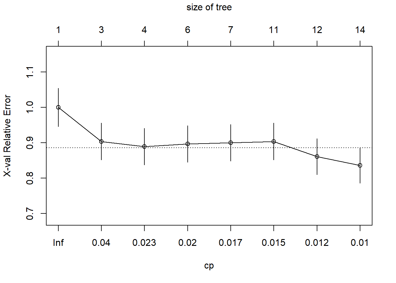
rpart.plot(vinoDT_prune, main="Wine Decision Tree") #plot tree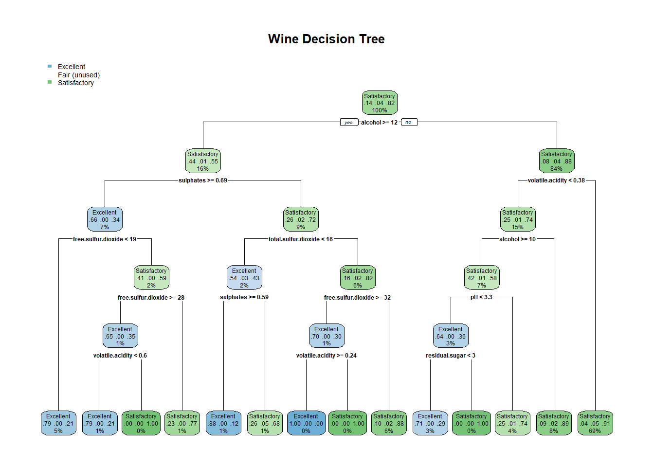
Here the accuracy of the model prediction is up to 88%. This method brought down the error rate in the false positive and false negative areas 34 down to 24 and 19 down to 11. A good result even above the C5.0 boosted output. This model optimized the error rate by cutting off the tree in the 8 area.
vinoDT_pred <- predict(vinoDT_prune, newdata = vinoDT_test, type = "class")
confusionMatrix(vinoDT_test$quality, vinoDT_pred, dnn = c('actual quality', 'predicted quality'))
## Confusion Matrix and Statistics
##
## predicted quality
## actual quality Excellent Fair Satisfactory
## Excellent 41 0 31
## Fair 0 0 21
## Satisfactory 8 0 379
##
## Overall Statistics
##
## Accuracy : 0.875
## 95% CI : (0.842, 0.9032)
## No Information Rate : 0.8979
## P-Value [Acc > NIR] : 0.9553
##
## Kappa : 0.5206
##
## Mcnemar's Test P-Value : NA
##
## Statistics by Class:
##
## Class: Excellent Class: Fair Class: Satisfactory
## Sensitivity 0.83673 NA 0.8794
## Specificity 0.92807 0.95625 0.8367
## Pos Pred Value 0.56944 NA 0.9793
## Neg Pred Value 0.98039 NA 0.4409
## Prevalence 0.10208 0.00000 0.8979
## Detection Rate 0.08542 0.00000 0.7896
## Detection Prevalence 0.15000 0.04375 0.8063
## Balanced Accuracy 0.88240 NA 0.8580plot(vinoDT_pred ~ quality, data=vinoDT_test, xlab="Actual", ylab = "Predicted")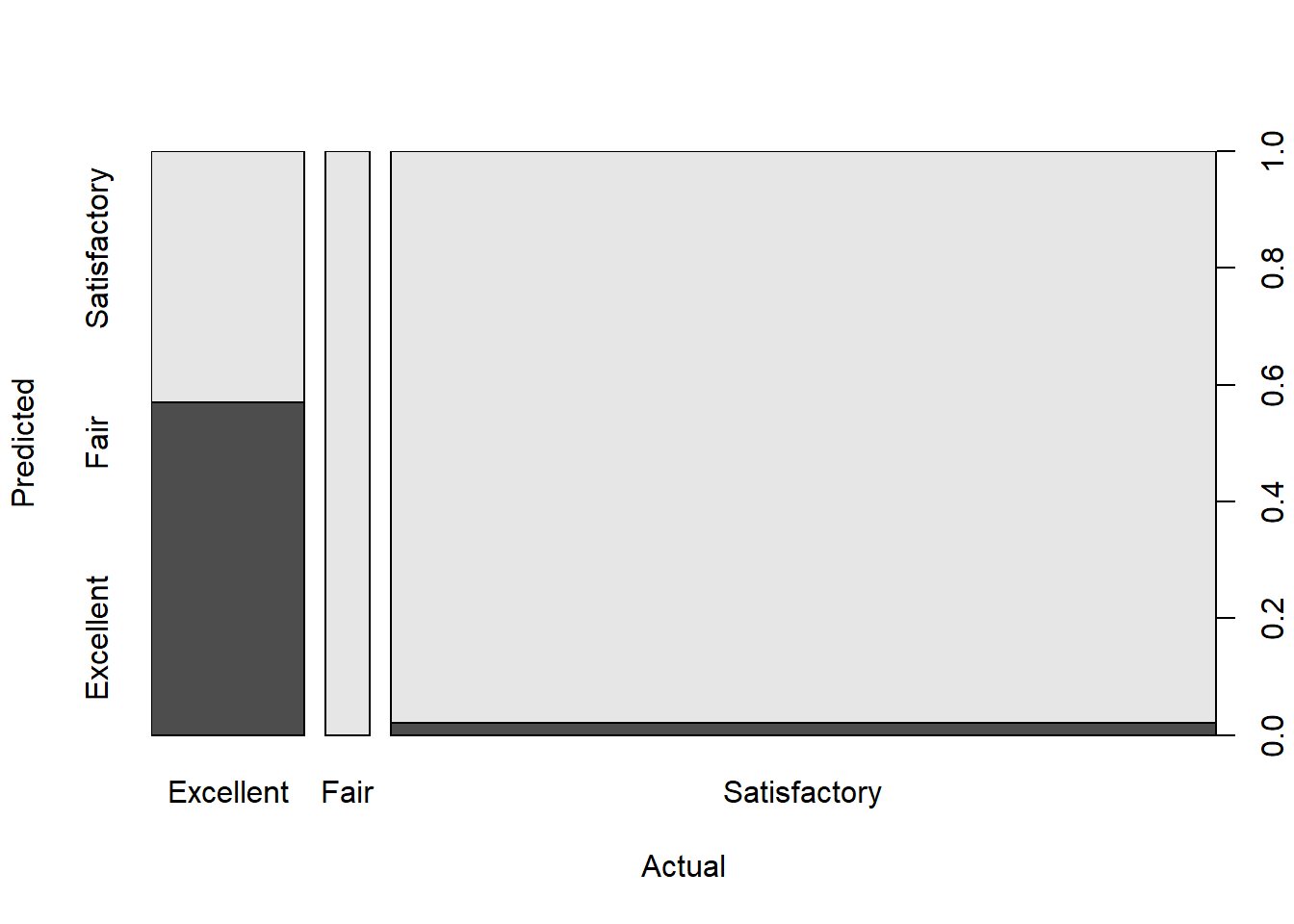
Random Forest
#Random Forest
#library(randomForest)
#Split data 70/30
set.seed(9876)
ind <- sample(1599, 1119) #70/30 data split
trainData <- vino1[ind, ] #training set
testData <- vino1[-ind, ] #testing set
rf <- randomForest(quality ~., data = trainData, ntree=100, proximity=TRUE)
table(predict(rf), trainData$quality)
##
## Excellent Fair Satisfactory
## Excellent 87 1 24
## Fair 0 0 0
## Satisfactory 72 43 892((rf)) #print ##
## Call:
## randomForest(formula = quality ~ ., data = trainData, ntree = 100, proximity = TRUE)
## Type of random forest: classification
## Number of trees: 100
## No. of variables tried at each split: 3
##
## OOB estimate of error rate: 12.51%
## Confusion matrix:
## Excellent Fair Satisfactory class.error
## Excellent 87 0 72 0.45283019
## Fair 1 0 43 1.00000000
## Satisfactory 24 0 892 0.02620087attributes(rf)## $names
## [1] "call" "type" "predicted" "err.rate"
## [5] "confusion" "votes" "oob.times" "classes"
## [9] "importance" "importanceSD" "localImportance" "proximity"
## [13] "ntree" "mtry" "forest" "y"
## [17] "test" "inbag" "terms"
##
## $class
## [1] "randomForest.formula" "randomForest"plot(rf)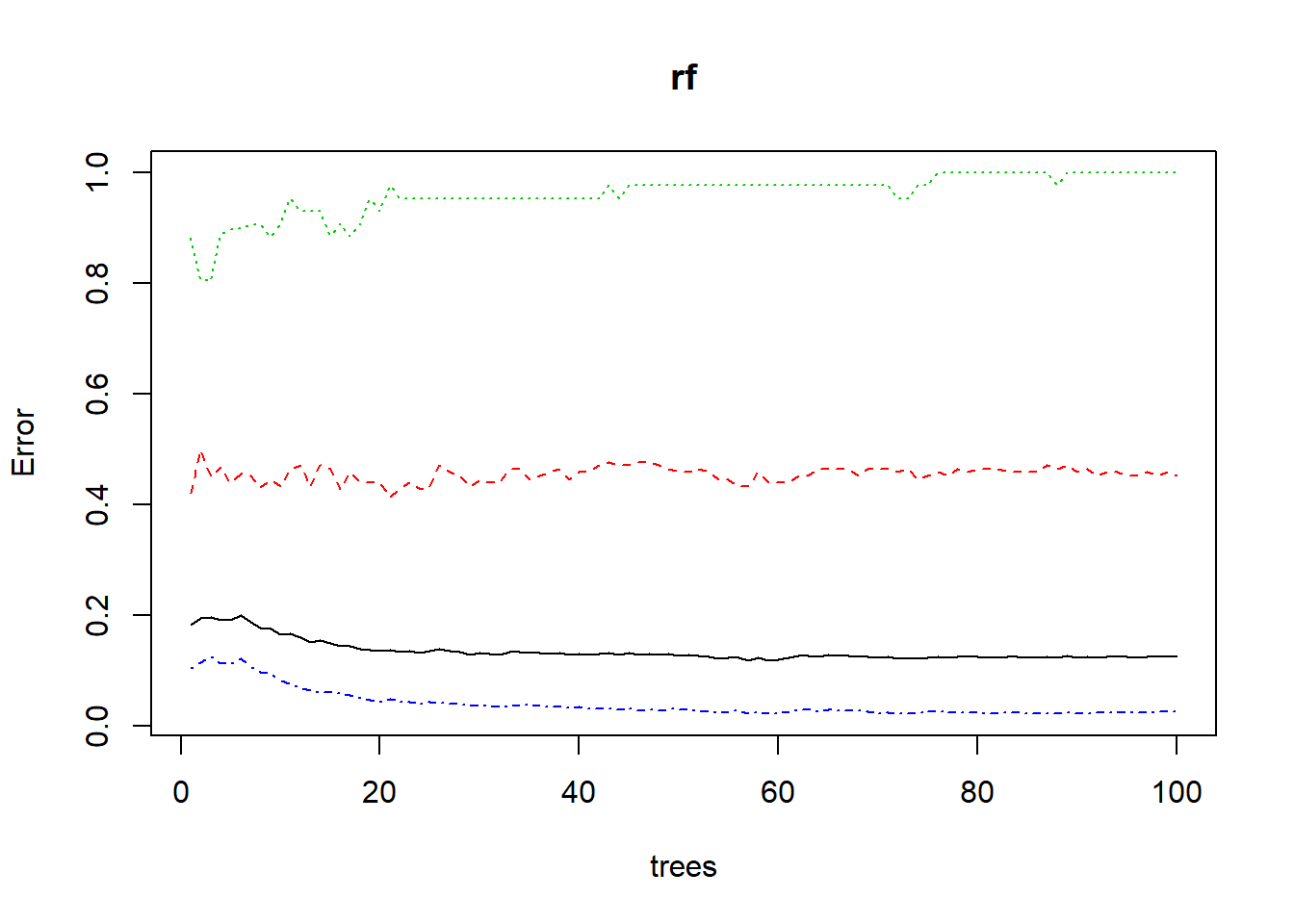 The random forest shows alcohol at 50.67 and volatile.acidity at 39.99 under the MeanDecrease which is similar to the decision tree is highest ranking. Some of the other variables are also similar we see pH not at the lowest at 24.68 but fee.sulfur.dioxide is lowest at 21.55 in this model. The preceding graph demonstrates the same numbers from the table.
importance(rf)## MeanDecreaseGini
## fixed.acidity 25.42739
## volatile.acidity 44.73501
## citric.acid 27.87692
## residual.sugar 25.44751
## chlorides 27.65742
## free.sulfur.dioxide 20.05222
## total.sulfur.dioxide 26.89442
## density 30.71208
## pH 22.67565
## sulphates 42.21175
## alcohol 50.04752varImpPlot(rf)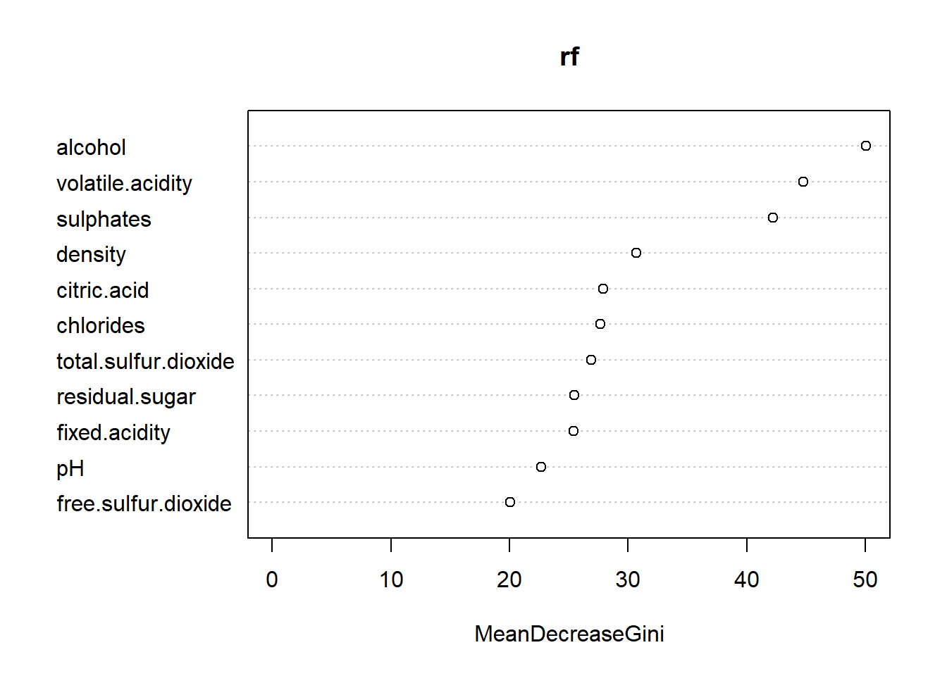
vinoPred <- predict(rf, newdata = testData, type = "class")
table(vinoPred, testData$quality)
##
## vinoPred Excellent Fair Satisfactory
## Excellent 22 0 12
## Fair 0 0 0
## Satisfactory 36 19 391This model shows an accuracy of 87% which is an increase from other models used.
confusionMatrix(testData$quality, vinoPred,dnn = c('actual', 'predicted'))## Confusion Matrix and Statistics
##
## predicted
## actual Excellent Fair Satisfactory
## Excellent 22 0 36
## Fair 0 0 19
## Satisfactory 12 0 391
##
## Overall Statistics
##
## Accuracy : 0.8604
## 95% CI : (0.8262, 0.8902)
## No Information Rate : 0.9292
## P-Value [Acc > NIR] : 1
##
## Kappa : 0.3395
##
## Mcnemar's Test P-Value : NA
##
## Statistics by Class:
##
## Class: Excellent Class: Fair Class: Satisfactory
## Sensitivity 0.64706 NA 0.8767
## Specificity 0.91928 0.96042 0.6471
## Pos Pred Value 0.37931 NA 0.9702
## Neg Pred Value 0.97156 NA 0.2857
## Prevalence 0.07083 0.00000 0.9292
## Detection Rate 0.04583 0.00000 0.8146
## Detection Prevalence 0.12083 0.03958 0.8396
## Balanced Accuracy 0.78317 NA 0.7619