K-Means Analysis
This project will use the Wholesale customer Data Set from: https://archive.ics.uci.edu/ml/datasets/Wholesale+customers. The data has 440 orbs and 8 variables. The data has the Channel and Region as integers but they are categorical in nature with 2 channels and 3 regions. We think this may need to be taken out of the analysis but will leave them in for now. A general observation about the variables there are outliers in the 6 major variables: fresh, milk, grocery, frozen, detergents_paper, delicassen. There are plot of each variable. In addition, to the outliers it is noted that the data is dense at the bottom of each of the variable graphs. “Fresh” seems to be less dense than the rest and “Delicassen” is the thickest density of points at the bottom. Initial thoughts are the clusters are going to be somewhere at the bottom of the graph.
library(stats)
library(fpc)
library(factoextra)
library(cluster)
library(fpc)
library(NbClust)
library(ggplot2)
Wholesale_customers_data = read.csv("https://archive.ics.uci.edu/ml/machine-learning-databases/00292/Wholesale%20customers%20data.csv", row.names=NULL)
df <- Wholesale_customers_datals(df)## [1] "Channel" "Delicassen" "Detergents_Paper" "Fresh"
## [5] "Frozen" "Grocery" "Milk" "Region"str(df)## 'data.frame': 440 obs. of 8 variables:
## $ Channel : int 2 2 2 1 2 2 2 2 1 2 ...
## $ Region : int 3 3 3 3 3 3 3 3 3 3 ...
## $ Fresh : int 12669 7057 6353 13265 22615 9413 12126 7579 5963 6006 ...
## $ Milk : int 9656 9810 8808 1196 5410 8259 3199 4956 3648 11093 ...
## $ Grocery : int 7561 9568 7684 4221 7198 5126 6975 9426 6192 18881 ...
## $ Frozen : int 214 1762 2405 6404 3915 666 480 1669 425 1159 ...
## $ Detergents_Paper: int 2674 3293 3516 507 1777 1795 3140 3321 1716 7425 ...
## $ Delicassen : int 1338 1776 7844 1788 5185 1451 545 2566 750 2098 ...summary(df)## Channel Region Fresh Milk
## Min. :1.000 Min. :1.000 Min. : 3 Min. : 55
## 1st Qu.:1.000 1st Qu.:2.000 1st Qu.: 3128 1st Qu.: 1533
## Median :1.000 Median :3.000 Median : 8504 Median : 3627
## Mean :1.323 Mean :2.543 Mean : 12000 Mean : 5796
## 3rd Qu.:2.000 3rd Qu.:3.000 3rd Qu.: 16934 3rd Qu.: 7190
## Max. :2.000 Max. :3.000 Max. :112151 Max. :73498
## Grocery Frozen Detergents_Paper Delicassen
## Min. : 3 Min. : 25.0 Min. : 3.0 Min. : 3.0
## 1st Qu.: 2153 1st Qu.: 742.2 1st Qu.: 256.8 1st Qu.: 408.2
## Median : 4756 Median : 1526.0 Median : 816.5 Median : 965.5
## Mean : 7951 Mean : 3071.9 Mean : 2881.5 Mean : 1524.9
## 3rd Qu.:10656 3rd Qu.: 3554.2 3rd Qu.: 3922.0 3rd Qu.: 1820.2
## Max. :92780 Max. :60869.0 Max. :40827.0 Max. :47943.0plot(df$Fresh)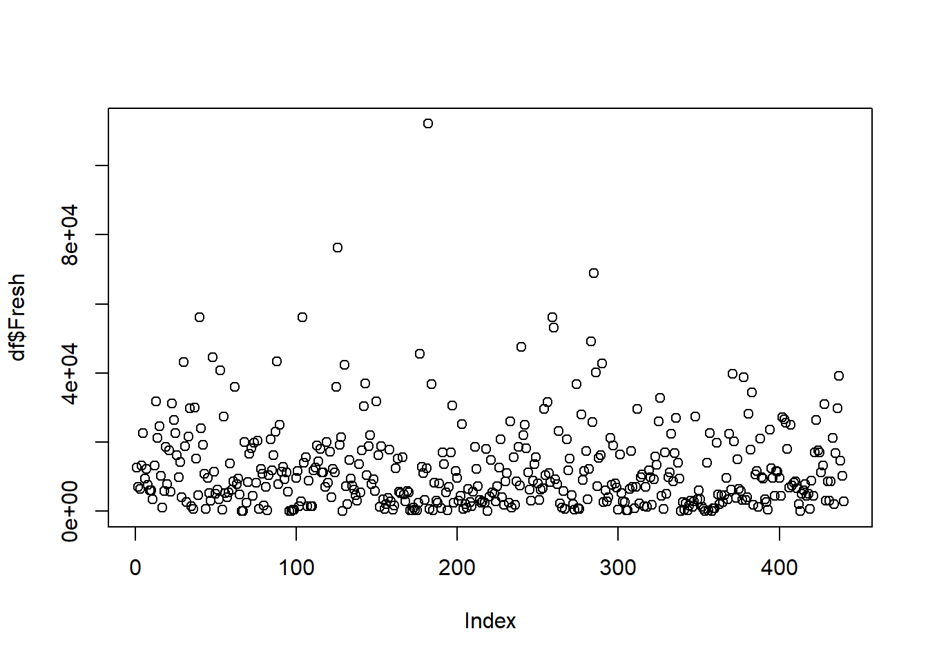
plot(df$Milk)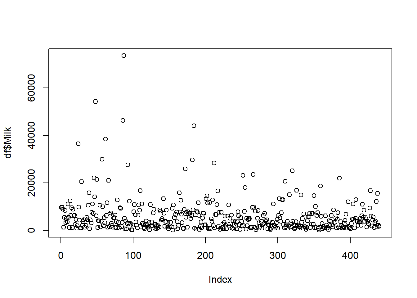
plot(df$Grocery)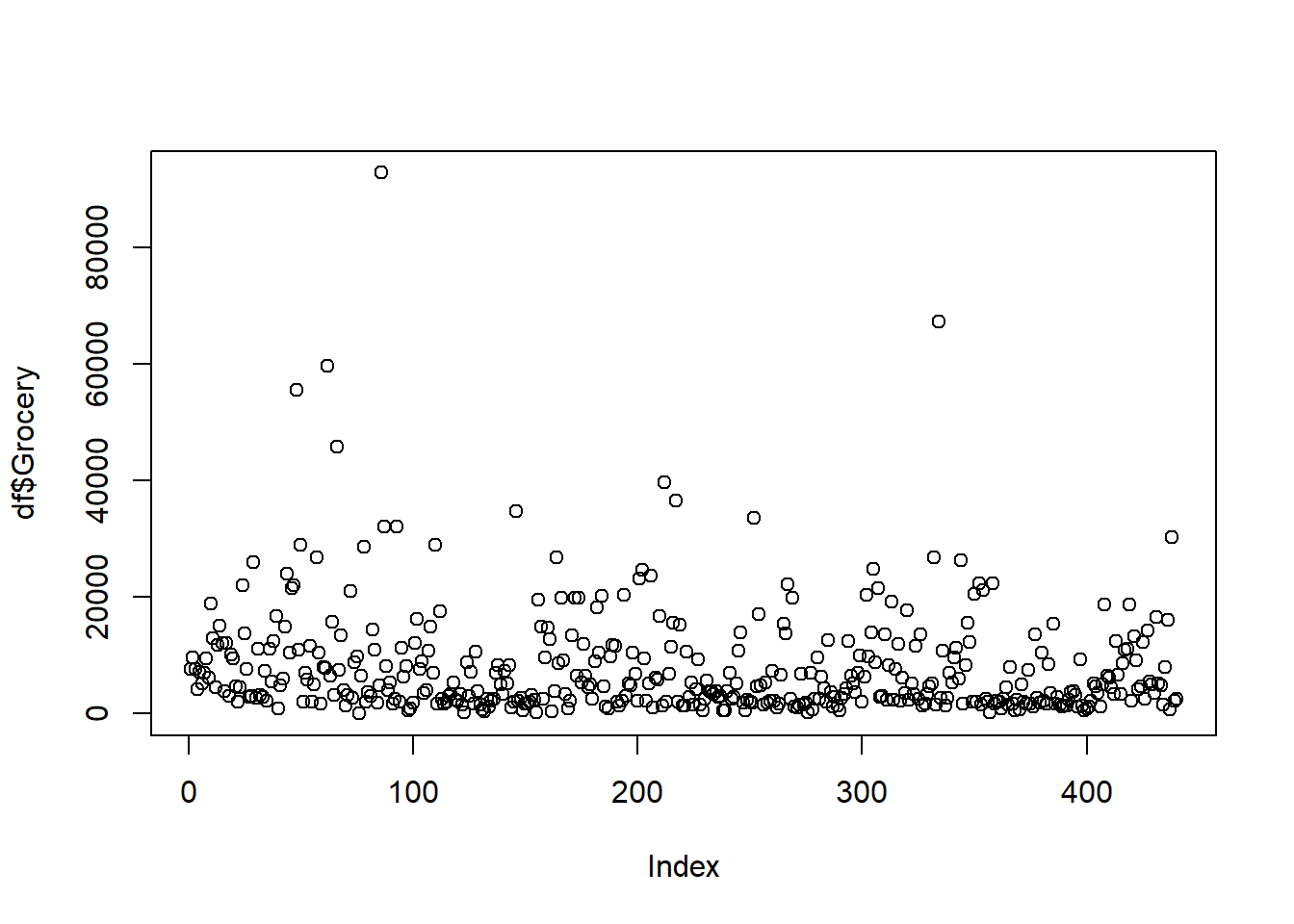
plot(df$Frozen)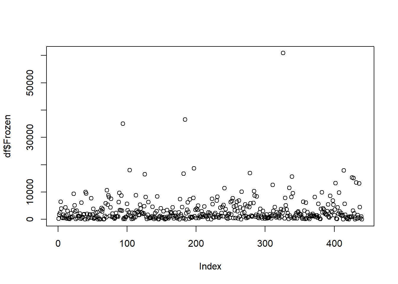
plot(df$Detergents_Paper)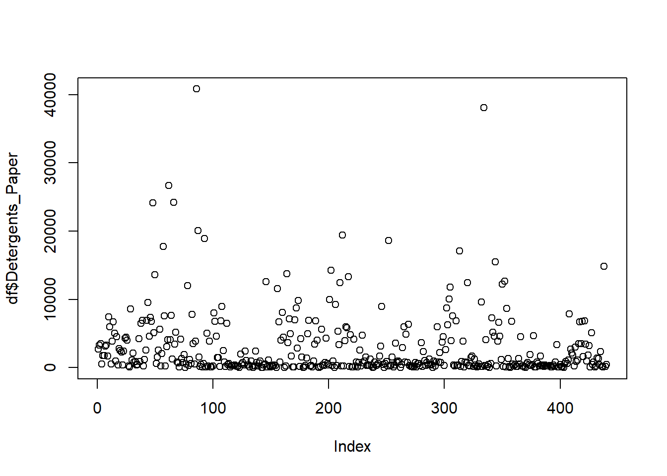
plot(df$Delicassen)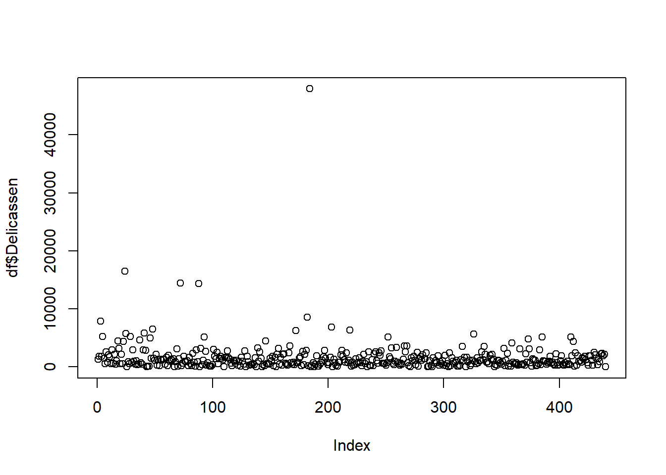
table(df$Channel)##
## 1 2
## 298 142table(df$Region)##
## 1 2 3
## 77 47 316groc <- dfThe data needs to be normalize or scaled since we have values of 1 to 112,151. It was assumed early on that the normalization function could be used, however, all of the different tutorials used the scale function which would give some values below 0 up to 16.45. This is not known why it is important to have negative values. Normalize would place everything in 0 to 1. Perhaps this would be too dense of the points?
# normalize <- function(x) {return ((x - min(x)) / (max(x) - min(x)))}
#df_z <- as.data.frame(lapply(df[c("Fresh", "Milk","Grocery","Frozen", "Detergents_Paper", "Delicassen")], normalize))
df_z <- as.data.frame(lapply(groc, scale))
summary(df_z)
## Channel Region Fresh Milk
## Min. :-0.6895 Min. :-1.9931 Min. :-0.9486 Min. :-0.7779
## 1st Qu.:-0.6895 1st Qu.:-0.7015 1st Qu.:-0.7015 1st Qu.:-0.5776
## Median :-0.6895 Median : 0.5900 Median :-0.2764 Median :-0.2939
## Mean : 0.0000 Mean : 0.0000 Mean : 0.0000 Mean : 0.0000
## 3rd Qu.: 1.4470 3rd Qu.: 0.5900 3rd Qu.: 0.3901 3rd Qu.: 0.1889
## Max. : 1.4470 Max. : 0.5900 Max. : 7.9187 Max. : 9.1732
## Grocery Frozen Detergents_Paper Delicassen
## Min. :-0.8364 Min. :-0.62763 Min. :-0.6037 Min. :-0.5396
## 1st Qu.:-0.6101 1st Qu.:-0.47988 1st Qu.:-0.5505 1st Qu.:-0.3960
## Median :-0.3363 Median :-0.31844 Median :-0.4331 Median :-0.1984
## Mean : 0.0000 Mean : 0.00000 Mean : 0.0000 Mean : 0.0000
## 3rd Qu.: 0.2846 3rd Qu.: 0.09935 3rd Qu.: 0.2182 3rd Qu.: 0.1047
## Max. : 8.9264 Max. :11.90545 Max. : 7.9586 Max. :16.4597plot(df_z$Channel, df_z$Fresh, main="Channel and Fresh")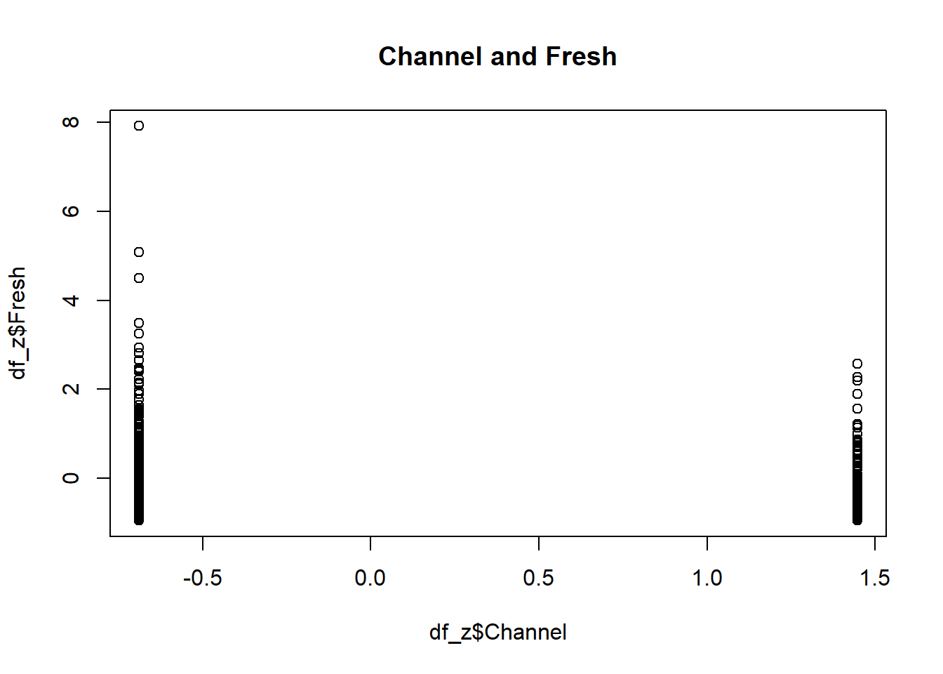
plot(df_z$Region, df_z$Fresh, main="Region and Fresh")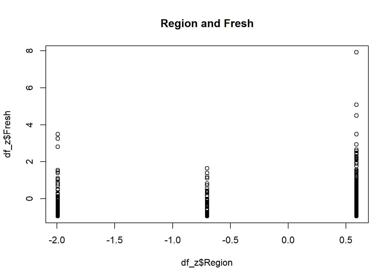
plot(df_z$Fresh, df_z$Grocery, main="Fresh and Grocery")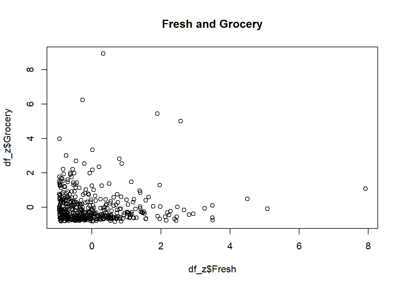
plot(df_z$Frozen, df_z$Grocery, main="Frozen and Grocery")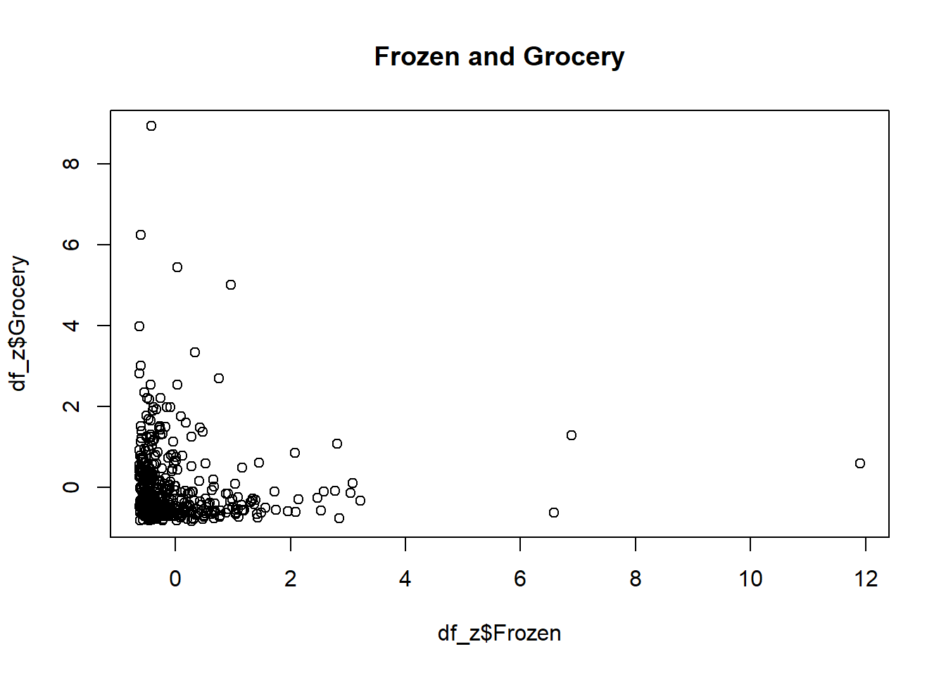
plot(df_z$Fresh, df_z$Delicassen, main="Fresh and Delicassen")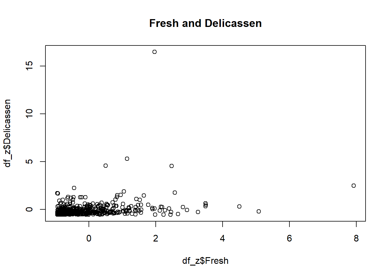
The K-Means is started here with a base of 2 clusters. and produces a 26.2% between sum of squares and total sum of squares ratio. We then look at the objects in the model and plot. In the first plot the two cluster points are close in the bottom right corner “X”, as speculated. Then to compare 5, 8 clusters are presented. The 5 cluster give a ratio of 56.2% and the 8 cluster gives a ratio of 69.7% which during testing was as high as 71%. Thus the within-cluster sum of squares of 26.2% is the lowest and better cluster.
set.seed(5678)
km.out <- kmeans(df_z, 2, nstart = 20)
km.out
## K-means clustering with 2 clusters of sizes 305, 135
##
## Cluster means:
## Channel Region Fresh Milk Grocery Frozen
## 1 -0.6334724 -0.04941902 0.1245579 -0.3357379 -0.4216872 0.1225824
## 2 1.4311785 0.11165038 -0.2814087 0.7585190 0.9527008 -0.2769455
## Detergents_Paper Delicassen
## 1 -0.4368095 -0.09157253
## 2 0.9868659 0.20688608
##
## Clustering vector:
## [1] 2 2 2 1 2 2 2 2 1 2 2 1 2 2 2 1 2 1 2 1 2 1 1 2 2 2 1 1 2 1 1 1 1 1 1 2 1
## [38] 2 2 1 1 1 2 2 2 2 2 2 2 2 1 1 1 2 1 1 2 2 1 1 2 2 2 2 1 2 1 2 1 1 1 1 1 1
## [75] 2 1 1 2 1 1 1 2 2 1 2 2 2 1 1 1 1 1 2 1 2 1 2 1 1 1 2 2 2 1 1 1 2 2 2 2 1
## [112] 2 1 1 1 1 1 1 1 1 1 1 1 2 1 1 1 2 1 1 1 1 1 1 1 1 1 1 1 1 1 1 1 1 1 2 1 1
## [149] 1 1 1 1 1 1 1 2 2 1 2 2 2 1 1 2 2 2 2 1 1 1 2 2 1 2 1 2 1 1 1 1 1 1 1 2 1
## [186] 1 1 1 2 2 1 1 1 2 1 1 1 2 1 1 2 2 1 1 1 2 1 2 1 2 1 2 1 1 2 1 2 1 2 1 1 1
## [223] 1 1 1 1 2 1 1 1 1 1 1 1 1 1 1 1 1 1 1 1 1 1 1 2 1 1 1 1 1 2 1 1 1 1 1 1 1
## [260] 1 1 1 1 1 2 1 2 1 2 1 1 1 1 1 1 1 1 1 1 2 1 2 1 1 1 1 1 1 1 1 1 1 1 2 1 2
## [297] 1 2 2 1 2 2 2 2 2 2 2 1 1 2 1 1 2 1 1 2 1 1 1 2 1 1 1 1 1 1 1 1 1 1 1 2 1
## [334] 2 1 2 1 1 1 1 2 2 1 2 1 1 2 2 1 2 1 2 1 2 1 1 1 2 1 1 1 1 1 1 1 2 1 1 1 1
## [371] 1 1 1 2 1 1 2 1 1 2 1 1 1 1 1 1 1 1 1 1 1 1 1 1 1 1 2 1 1 1 1 1 1 1 1 1 1
## [408] 2 2 1 1 1 1 1 1 2 2 1 2 1 1 2 1 1 2 1 1 1 1 1 1 1 1 1 1 1 1 2 1 1
##
## Within cluster sum of squares by cluster:
## [1] 1315.784 1277.692
## (between_SS / total_SS = 26.2 %)
##
## Available components:
##
## [1] "cluster" "centers" "totss" "withinss" "tot.withinss"
## [6] "betweenss" "size" "iter" "ifault"plot(df_z$Fresh, col=(km.out$cluster+3), main="K-means clustering results with K=2", xlab="", ylab="", pch=1.25, cex=1)
points(km.out$centers[,c("Fresh", "Frozen")], pch=1, cex=3, col="red", lwd=2)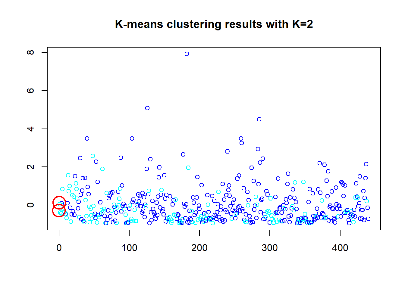
set.seed(5679)
km.out <- kmeans(df_z, 5, nstart = 20)
km.out
## K-means clustering with 5 clusters of sizes 91, 210, 10, 126, 3
##
## Cluster means:
## Channel Region Fresh Milk Grocery Frozen
## 1 -0.5721212 -1.59567800 0.01452064 -0.3443661 -0.4020087 0.079577121
## 2 -0.6793383 0.58999669 0.11253552 -0.3555734 -0.4424744 0.073160058
## 3 1.4470045 -0.05577083 0.31347349 3.9174467 4.2707490 -0.003570131
## 4 1.4470045 0.16973529 -0.31436434 0.4519519 0.6653892 -0.350667521
## 5 -0.6895122 0.15948501 3.84044484 3.2957757 0.9852919 7.204892918
## Detergents_Paper Delicassen
## 1 -0.4239285 -0.13295117
## 2 -0.4432338 -0.09138933
## 3 4.6129149 0.50279301
## 4 0.6824271 0.04653468
## 5 -0.1527927 6.79967230
##
## Clustering vector:
## [1] 4 4 4 2 4 4 4 4 2 4 4 4 4 4 4 2 4 2 4 2 4 2 2 4 4 4 2 2 4 2 2 2 2 2 2 4 2
## [38] 4 4 2 2 2 4 4 4 4 4 3 4 4 2 2 4 4 2 2 3 4 2 2 4 3 4 4 2 3 2 4 2 2 2 2 2 4
## [75] 4 2 2 4 2 2 2 4 4 2 4 3 3 2 2 2 2 2 3 2 4 2 4 2 2 2 4 4 4 2 2 2 4 4 4 4 2
## [112] 4 2 2 2 2 2 2 2 2 2 2 2 4 2 2 2 4 2 2 2 2 2 2 2 2 2 2 2 2 2 2 2 2 2 4 2 2
## [149] 2 2 2 2 2 2 2 4 4 2 4 4 4 2 2 4 4 4 4 2 2 2 4 4 2 4 2 4 2 2 2 2 2 5 2 5 2
## [186] 2 2 2 4 4 2 2 2 4 2 2 1 4 1 1 4 4 1 1 1 4 1 1 1 4 1 3 1 1 4 1 4 1 4 1 1 1
## [223] 1 1 1 1 1 1 1 1 1 1 1 1 1 1 1 1 1 1 1 1 1 1 1 4 1 1 1 1 1 3 1 1 1 1 1 1 1
## [260] 1 1 1 1 1 4 1 4 1 4 1 1 1 1 2 2 2 2 2 2 4 2 4 2 2 2 2 2 2 2 2 2 2 2 4 1 4
## [297] 1 4 4 1 4 4 4 4 4 4 4 1 1 4 1 1 4 1 1 4 1 1 1 4 1 1 1 1 1 5 1 1 1 1 1 4 1
## [334] 3 1 4 1 1 1 1 4 4 2 4 2 2 4 4 2 4 2 4 2 4 2 2 2 4 2 2 2 2 2 2 2 4 2 2 2 2
## [371] 2 2 2 4 2 2 4 2 2 4 2 2 2 2 2 2 2 2 2 2 2 2 2 2 2 2 4 2 2 2 2 2 2 2 2 2 2
## [408] 4 4 2 2 2 2 2 2 4 4 2 4 2 2 4 2 4 4 2 2 2 2 2 2 2 2 2 2 2 2 4 2 2
##
## Within cluster sum of squares by cluster:
## [1] 221.0813 541.8922 160.2905 398.3096 215.6517
## (between_SS / total_SS = 56.2 %)
##
## Available components:
##
## [1] "cluster" "centers" "totss" "withinss" "tot.withinss"
## [6] "betweenss" "size" "iter" "ifault"plot(df_z$Fresh, col=(km.out$cluster+1), main="K-means clustering results with K=5", xlab="", ylab="", pch=1.25, cex=1)
points(km.out$centers[,c("Fresh", "Frozen")], pch=1, cex=3, col="red", lwd=2)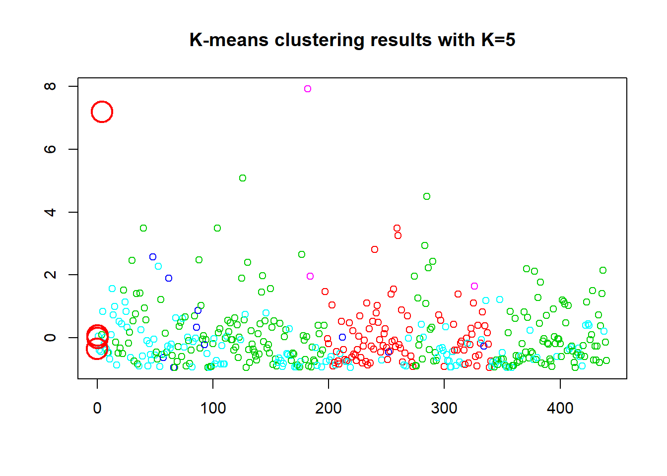
set.seed(5671)
km.out <- kmeans(df_z, 8, nstart = 20)
km.out
## K-means clustering with 8 clusters of sizes 36, 156, 5, 1, 5, 85, 59, 93
##
## Cluster means:
## Channel Region Fresh Milk Grocery Frozen
## 1 1.4470045 -0.5221585 -0.4928922 1.3582881 1.7487863 -0.28074063
## 2 -0.6895122 0.5899967 -0.3416985 -0.3904737 -0.4688299 -0.21071338
## 3 1.4470045 0.3316897 1.0755395 5.1033075 5.6319063 -0.08979632
## 4 -0.6895122 0.5899967 1.9645810 5.1696185 1.2857533 6.89275382
## 5 -0.6895122 0.3316897 3.6134035 0.7451291 0.2123001 5.43102828
## 6 -0.5638348 -1.6132101 -0.1569262 -0.3436053 -0.3976095 0.01054604
## 7 -0.5808758 0.3492020 1.4339190 -0.2537941 -0.3715451 0.69869430
## 8 1.4470045 0.4233470 -0.2755129 0.2342368 0.3805628 -0.35204667
## Detergents_Paper Delicassen
## 1 1.8447981 0.34264536
## 2 -0.4329138 -0.18642642
## 3 5.6823687 0.41981740
## 4 -0.5542311 16.45971129
## 5 -0.2457485 0.89703352
## 6 -0.4107407 -0.15629362
## 7 -0.4685727 0.17667111
## 8 0.3984054 -0.03693887
##
## Clustering vector:
## [1] 8 8 8 2 8 8 8 8 2 8 8 8 8 8 8 2 8 2 8 2 8 2 7 1 8 8 2 2 1 7 2 2 2 7 2 8 7
## [38] 8 8 7 7 2 8 1 8 1 8 3 8 1 2 2 7 8 7 2 1 8 2 2 8 3 8 8 2 1 2 8 2 2 7 7 2 8
## [75] 8 7 2 1 2 2 2 8 8 2 8 3 3 7 2 7 2 2 1 5 8 2 8 2 2 2 8 8 8 5 2 2 8 8 8 8 2
## [112] 8 7 2 2 2 2 2 7 2 2 2 2 8 7 5 7 8 2 7 2 2 2 2 2 2 2 2 2 2 2 7 7 2 2 1 2 2
## [149] 2 7 2 2 2 2 2 1 8 2 8 8 8 2 2 1 8 8 8 2 2 2 8 1 2 8 2 8 7 2 2 2 2 5 2 4 2
## [186] 2 2 2 8 8 7 2 2 8 2 7 7 6 6 6 1 1 6 6 6 1 6 6 6 1 6 1 6 6 8 6 1 6 1 6 6 6
## [223] 6 6 6 6 6 6 6 6 6 6 6 6 6 6 6 6 6 7 6 6 6 6 6 1 6 6 6 6 6 1 6 6 6 6 6 6 7
## [260] 7 6 6 6 6 1 6 1 6 1 6 6 6 6 7 2 2 7 7 2 8 2 8 7 7 7 7 2 7 2 7 2 2 2 8 6 8
## [297] 6 8 8 6 8 1 8 8 1 8 1 6 6 1 6 7 1 6 6 8 6 6 6 1 6 6 6 6 7 5 6 6 6 6 6 1 6
## [334] 3 7 8 6 6 6 6 8 8 2 1 2 2 8 8 2 1 2 1 2 8 2 2 7 8 2 2 2 2 2 2 2 8 2 2 2 2
## [371] 7 7 2 8 2 2 8 7 2 8 7 7 7 2 2 2 2 2 2 2 2 2 2 7 2 2 8 2 2 2 2 7 7 7 2 2 7
## [408] 8 8 2 2 2 2 7 2 8 8 2 8 2 2 8 7 8 8 7 2 7 2 2 2 7 2 2 2 7 7 1 2 2
##
## Within cluster sum of squares by cluster:
## [1] 190.61080 129.76038 92.86852 0.00000 119.17144 165.34225 229.77076
## [8] 137.67863
## (between_SS / total_SS = 69.7 %)
##
## Available components:
##
## [1] "cluster" "centers" "totss" "withinss" "tot.withinss"
## [6] "betweenss" "size" "iter" "ifault"set.seed(4567)
km.out <- kmeans(df_z, 8, nstart = 50)
km.out## K-means clustering with 8 clusters of sizes 5, 59, 156, 36, 85, 1, 5, 93
##
## Cluster means:
## Channel Region Fresh Milk Grocery Frozen
## 1 1.4470045 0.3316897 1.0755395 5.1033075 5.6319063 -0.08979632
## 2 -0.5808758 0.3492020 1.4339190 -0.2537941 -0.3715451 0.69869430
## 3 -0.6895122 0.5899967 -0.3416985 -0.3904737 -0.4688299 -0.21071338
## 4 1.4470045 -0.5221585 -0.4928922 1.3582881 1.7487863 -0.28074063
## 5 -0.5638348 -1.6132101 -0.1569262 -0.3436053 -0.3976095 0.01054604
## 6 -0.6895122 0.5899967 1.9645810 5.1696185 1.2857533 6.89275382
## 7 -0.6895122 0.3316897 3.6134035 0.7451291 0.2123001 5.43102828
## 8 1.4470045 0.4233470 -0.2755129 0.2342368 0.3805628 -0.35204667
## Detergents_Paper Delicassen
## 1 5.6823687 0.41981740
## 2 -0.4685727 0.17667111
## 3 -0.4329138 -0.18642642
## 4 1.8447981 0.34264536
## 5 -0.4107407 -0.15629362
## 6 -0.5542311 16.45971129
## 7 -0.2457485 0.89703352
## 8 0.3984054 -0.03693887
##
## Clustering vector:
## [1] 8 8 8 3 8 8 8 8 3 8 8 8 8 8 8 3 8 3 8 3 8 3 2 4 8 8 3 3 4 2 3 3 3 2 3 8 2
## [38] 8 8 2 2 3 8 4 8 4 8 1 8 4 3 3 2 8 2 3 4 8 3 3 8 1 8 8 3 4 3 8 3 3 2 2 3 8
## [75] 8 2 3 4 3 3 3 8 8 3 8 1 1 2 3 2 3 3 4 7 8 3 8 3 3 3 8 8 8 7 3 3 8 8 8 8 3
## [112] 8 2 3 3 3 3 3 2 3 3 3 3 8 2 7 2 8 3 2 3 3 3 3 3 3 3 3 3 3 3 2 2 3 3 4 3 3
## [149] 3 2 3 3 3 3 3 4 8 3 8 8 8 3 3 4 8 8 8 3 3 3 8 4 3 8 3 8 2 3 3 3 3 7 3 6 3
## [186] 3 3 3 8 8 2 3 3 8 3 2 2 5 5 5 4 4 5 5 5 4 5 5 5 4 5 4 5 5 8 5 4 5 4 5 5 5
## [223] 5 5 5 5 5 5 5 5 5 5 5 5 5 5 5 5 5 2 5 5 5 5 5 4 5 5 5 5 5 4 5 5 5 5 5 5 2
## [260] 2 5 5 5 5 4 5 4 5 4 5 5 5 5 2 3 3 2 2 3 8 3 8 2 2 2 2 3 2 3 2 3 3 3 8 5 8
## [297] 5 8 8 5 8 4 8 8 4 8 4 5 5 4 5 2 4 5 5 8 5 5 5 4 5 5 5 5 2 7 5 5 5 5 5 4 5
## [334] 1 2 8 5 5 5 5 8 8 3 4 3 3 8 8 3 4 3 4 3 8 3 3 2 8 3 3 3 3 3 3 3 8 3 3 3 3
## [371] 2 2 3 8 3 3 8 2 3 8 2 2 2 3 3 3 3 3 3 3 3 3 3 2 3 3 8 3 3 3 3 2 2 2 3 3 2
## [408] 8 8 3 3 3 3 2 3 8 8 3 8 3 3 8 2 8 8 2 3 2 3 3 3 2 3 3 3 2 2 4 3 3
##
## Within cluster sum of squares by cluster:
## [1] 92.86852 229.77076 129.76038 190.61080 165.34225 0.00000 119.17144
## [8] 137.67863
## (between_SS / total_SS = 69.7 %)
##
## Available components:
##
## [1] "cluster" "centers" "totss" "withinss" "tot.withinss"
## [6] "betweenss" "size" "iter" "ifault"Here we wanted to see what would happen if the “Channel” and “Region” are dropped and just the remaining 6 variables are used. And 2 clusters dropped the WCSS down to 26% even with cluster centers still in bottom left corner. The other clusters; k=6 has a 65.1% ratio sum of squares, and the k=8 increased WCSS to 71.7%. Thus 2 clusters maybe the best option. However, everything is compressed down in the bottom left corner, this seems hard to see what is going on visually in a scatter plot. Maybe not the best data set to use for an introductory exercise. We will use one more method to determine the optimal cluster number below.
groc <- df[3:8]
df_t <- as.data.frame(lapply(groc, scale))
set.seed(4568)
km.out1 <- kmeans(df_t, 2, nstart = 20)
km.out1## K-means clustering with 2 clusters of sizes 399, 41
##
## Cluster means:
## Fresh Milk Grocery Frozen Detergents_Paper Delicassen
## 1 -0.00542930 -0.2122882 -0.2302493 -0.03310806 -0.2320799 -0.0826124
## 2 0.05283636 2.0659269 2.2407190 0.32219794 2.2585338 0.8039597
##
## Clustering vector:
## [1] 1 1 1 1 1 1 1 1 1 1 1 1 1 1 1 1 1 1 1 1 1 1 1 2 1 1 1 1 2 1 1 1 1 1 1 1 1
## [38] 1 1 1 1 1 1 2 1 2 2 2 1 2 1 1 1 1 1 1 2 1 1 1 1 2 1 1 1 2 1 1 1 1 1 1 1 1
## [75] 1 1 1 2 1 1 1 1 1 1 1 2 2 1 1 1 1 1 2 1 1 1 1 1 1 1 1 1 1 1 1 1 1 1 1 1 1
## [112] 1 1 1 1 1 1 1 1 1 1 1 1 1 1 1 1 1 1 1 1 1 1 1 1 1 1 1 1 1 1 1 1 1 1 2 1 1
## [149] 1 1 1 1 1 1 1 2 1 1 1 1 1 1 1 2 1 2 1 1 1 1 1 2 1 1 1 1 1 1 1 1 1 2 1 2 1
## [186] 1 1 1 1 1 1 1 1 1 1 1 1 1 1 1 2 2 1 1 1 2 1 1 1 2 1 2 1 1 1 1 2 1 1 1 1 1
## [223] 1 1 1 1 1 1 1 1 1 1 1 1 1 1 1 1 1 1 1 1 1 1 1 1 1 1 1 1 1 2 1 1 1 1 1 1 1
## [260] 1 1 1 1 1 1 1 1 1 1 1 1 1 1 1 1 1 1 1 1 1 1 1 1 1 1 1 1 1 1 1 1 1 1 1 1 1
## [297] 1 1 1 1 1 2 1 1 2 1 2 1 1 2 1 1 2 1 1 1 1 1 1 2 1 1 1 1 1 2 1 1 1 1 1 2 1
## [334] 2 1 1 1 1 1 1 1 1 1 2 1 1 1 1 1 2 1 2 1 1 1 1 1 1 1 1 1 1 1 1 1 1 1 1 1 1
## [371] 1 1 1 1 1 1 1 1 1 1 1 1 1 1 1 1 1 1 1 1 1 1 1 1 1 1 1 1 1 1 1 1 1 1 1 1 1
## [408] 1 1 1 1 1 1 1 1 1 1 1 1 1 1 1 1 1 1 1 1 1 1 1 1 1 1 1 1 1 1 2 1 1
##
## Within cluster sum of squares by cluster:
## [1] 982.9619 966.3860
## (between_SS / total_SS = 26.0 %)
##
## Available components:
##
## [1] "cluster" "centers" "totss" "withinss" "tot.withinss"
## [6] "betweenss" "size" "iter" "ifault"plot(df_z$Fresh, col=(km.out1$cluster+3), main="K-means clustering results with K=2", xlab="", ylab="", pch=1.25, cex=1)
points(km.out1$centers[,c("Fresh", "Frozen")], pch=1, cex=3, col="red", lwd=2)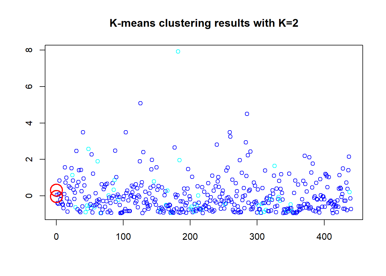
set.seed(4569)
km.out1
## K-means clustering with 2 clusters of sizes 399, 41
##
## Cluster means:
## Fresh Milk Grocery Frozen Detergents_Paper Delicassen
## 1 -0.00542930 -0.2122882 -0.2302493 -0.03310806 -0.2320799 -0.0826124
## 2 0.05283636 2.0659269 2.2407190 0.32219794 2.2585338 0.8039597
##
## Clustering vector:
## [1] 1 1 1 1 1 1 1 1 1 1 1 1 1 1 1 1 1 1 1 1 1 1 1 2 1 1 1 1 2 1 1 1 1 1 1 1 1
## [38] 1 1 1 1 1 1 2 1 2 2 2 1 2 1 1 1 1 1 1 2 1 1 1 1 2 1 1 1 2 1 1 1 1 1 1 1 1
## [75] 1 1 1 2 1 1 1 1 1 1 1 2 2 1 1 1 1 1 2 1 1 1 1 1 1 1 1 1 1 1 1 1 1 1 1 1 1
## [112] 1 1 1 1 1 1 1 1 1 1 1 1 1 1 1 1 1 1 1 1 1 1 1 1 1 1 1 1 1 1 1 1 1 1 2 1 1
## [149] 1 1 1 1 1 1 1 2 1 1 1 1 1 1 1 2 1 2 1 1 1 1 1 2 1 1 1 1 1 1 1 1 1 2 1 2 1
## [186] 1 1 1 1 1 1 1 1 1 1 1 1 1 1 1 2 2 1 1 1 2 1 1 1 2 1 2 1 1 1 1 2 1 1 1 1 1
## [223] 1 1 1 1 1 1 1 1 1 1 1 1 1 1 1 1 1 1 1 1 1 1 1 1 1 1 1 1 1 2 1 1 1 1 1 1 1
## [260] 1 1 1 1 1 1 1 1 1 1 1 1 1 1 1 1 1 1 1 1 1 1 1 1 1 1 1 1 1 1 1 1 1 1 1 1 1
## [297] 1 1 1 1 1 2 1 1 2 1 2 1 1 2 1 1 2 1 1 1 1 1 1 2 1 1 1 1 1 2 1 1 1 1 1 2 1
## [334] 2 1 1 1 1 1 1 1 1 1 2 1 1 1 1 1 2 1 2 1 1 1 1 1 1 1 1 1 1 1 1 1 1 1 1 1 1
## [371] 1 1 1 1 1 1 1 1 1 1 1 1 1 1 1 1 1 1 1 1 1 1 1 1 1 1 1 1 1 1 1 1 1 1 1 1 1
## [408] 1 1 1 1 1 1 1 1 1 1 1 1 1 1 1 1 1 1 1 1 1 1 1 1 1 1 1 1 1 1 2 1 1
##
## Within cluster sum of squares by cluster:
## [1] 982.9619 966.3860
## (between_SS / total_SS = 26.0 %)
##
## Available components:
##
## [1] "cluster" "centers" "totss" "withinss" "tot.withinss"
## [6] "betweenss" "size" "iter" "ifault"plot(df_z$Fresh, col=(km.out1$cluster+2), main="K-means clustering results with K=6", xlab="", ylab="", pch=1, cex=1)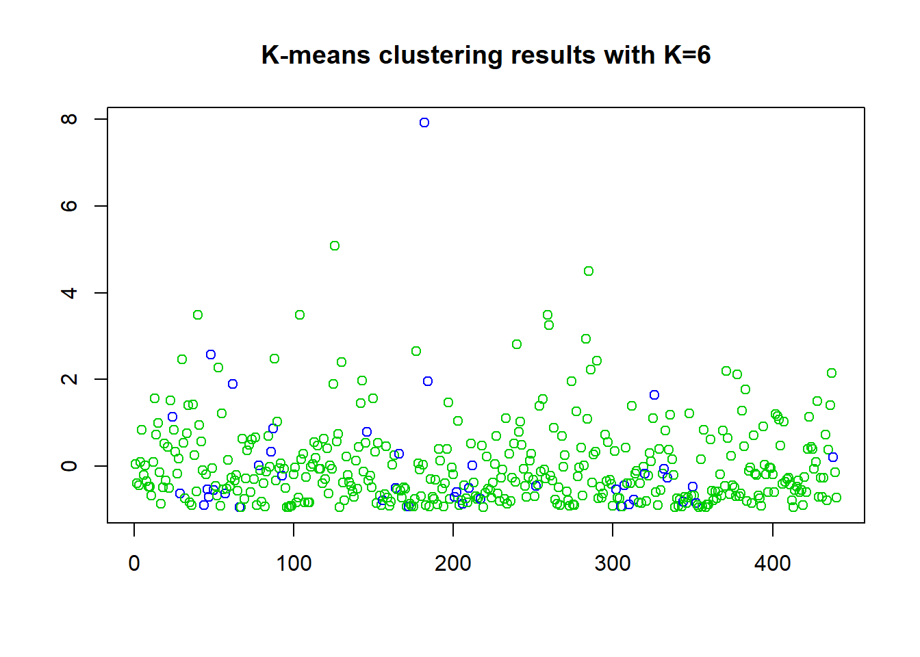
set.seed(4562)
km.out1 <- kmeans(df_t, 6, nstart = 20)
km.out1
## K-means clustering with 6 clusters of sizes 242, 88, 10, 94, 1, 5
##
## Cluster means:
## Fresh Milk Grocery Frozen Detergents_Paper Delicassen
## 1 -0.3472255 -0.3886643 -0.4345878 -0.182611380 -0.3885364 -0.21489822
## 2 1.2297852 -0.2212199 -0.2997703 0.471366329 -0.4171626 0.19696794
## 3 0.3134735 3.9174467 4.2707490 -0.003570131 4.6129149 0.50279301
## 4 -0.5038176 0.6963232 0.9201628 -0.332983798 0.9190419 0.09254661
## 5 1.9645810 5.1696185 1.2857533 6.892753825 -0.5542311 16.45971129
## 6 3.6134035 0.7451291 0.2123001 5.431028285 -0.2457485 0.89703352
##
## Clustering vector:
## [1] 1 4 4 1 2 1 1 1 1 4 4 1 2 4 4 1 4 1 2 1 1 1 2 4 2 1 1 1 4 2 2 1 1 2 1 1 2
## [38] 4 4 2 2 2 4 4 4 4 4 3 4 4 1 1 2 4 2 1 3 4 1 1 1 3 1 4 1 3 1 4 1 1 2 2 1 2
## [75] 1 2 1 4 1 1 1 4 4 2 1 3 3 2 1 2 1 1 3 6 4 1 1 1 1 1 4 4 1 6 1 1 4 4 1 4 1
## [112] 4 2 1 1 1 1 1 2 1 1 1 1 1 2 6 2 2 1 2 1 1 1 1 1 1 1 1 1 1 2 2 2 1 1 4 1 1
## [149] 1 2 1 1 1 1 1 4 4 1 1 4 4 1 1 4 1 4 4 1 1 1 4 4 1 4 1 4 2 1 1 1 1 6 4 5 1
## [186] 1 1 1 4 4 2 1 1 4 1 2 2 4 1 1 4 4 2 1 1 4 1 1 1 4 1 3 1 1 4 4 4 1 4 1 1 4
## [223] 1 1 1 1 2 1 1 1 1 1 2 1 1 1 1 2 1 2 2 2 1 1 4 4 1 1 1 1 1 3 1 2 4 2 1 1 2
## [260] 2 1 1 2 1 4 4 4 2 4 1 1 1 1 2 1 1 2 2 1 1 1 1 2 2 2 2 1 2 1 2 1 1 1 4 2 1
## [297] 1 1 1 1 1 4 4 4 4 4 4 1 1 4 1 2 4 1 1 4 1 1 1 4 1 1 1 1 2 6 1 1 2 1 1 4 2
## [334] 3 2 2 1 1 1 1 4 4 1 4 1 1 4 2 1 4 1 4 1 4 2 1 2 4 1 1 1 1 1 1 1 1 1 1 2 1
## [371] 2 2 1 1 1 1 4 2 1 1 2 2 2 1 4 1 1 2 1 1 1 1 1 2 1 1 4 1 1 1 1 2 2 2 2 1 2
## [408] 4 1 1 1 1 1 2 1 1 4 1 4 1 4 1 2 1 1 2 4 2 1 1 1 2 1 1 1 2 2 4 1 1
##
## Within cluster sum of squares by cluster:
## [1] 187.7405 240.9513 149.4481 224.3460 0.0000 117.8370
## (between_SS / total_SS = 65.1 %)
##
## Available components:
##
## [1] "cluster" "centers" "totss" "withinss" "tot.withinss"
## [6] "betweenss" "size" "iter" "ifault"set.seed(4561)
km.out1 <- kmeans(df_t, 8, nstart = 20)
km.out1## K-means clustering with 8 clusters of sizes 42, 2, 28, 41, 98, 5, 1, 223
##
## Cluster means:
## Fresh Milk Grocery Frozen Detergents_Paper Delicassen
## 1 0.2221728 -0.2896876 -0.42682693 1.43519472 -0.5011524 -0.04768952
## 2 0.7918828 0.5610464 -0.01128859 9.24203651 -0.4635194 0.93210312
## 3 -0.4453660 1.5449634 1.95334680 -0.25357812 2.1391487 0.38983626
## 4 2.2141700 -0.1367268 -0.16118733 0.32383076 -0.3593641 0.41697371
## 5 -0.4883343 0.4118988 0.50256612 -0.31004906 0.4748524 0.01870206
## 6 1.0755395 5.1033075 5.63190631 -0.08979632 5.6823687 0.41981740
## 7 1.9645810 5.1696185 1.28575327 6.89275382 -0.5542311 16.45971129
## 8 -0.2184362 -0.4379401 -0.48803805 -0.27353403 -0.4375782 -0.21643132
##
## Clustering vector:
## [1] 5 5 5 1 4 8 8 5 8 5 5 8 4 5 5 8 5 8 5 8 8 8 4 3 5 8 8 8 3 4 8 8 8 4 8 5 4
## [38] 5 5 4 1 8 5 3 5 3 5 6 5 3 8 8 4 5 4 8 3 5 8 5 8 6 5 5 8 3 8 5 8 8 1 4 1 1
## [75] 5 8 1 3 8 8 8 5 5 8 8 6 6 4 1 4 8 1 3 2 5 8 8 8 8 8 5 5 5 4 8 8 5 5 5 5 8
## [112] 5 1 8 8 8 8 8 1 8 8 8 8 5 4 4 1 5 8 4 8 8 8 8 8 8 5 8 8 8 8 4 4 1 8 3 8 8
## [149] 8 4 8 8 8 8 8 3 5 8 5 5 5 8 8 3 5 5 5 8 8 8 5 3 8 5 8 5 4 8 8 8 8 4 5 7 8
## [186] 8 8 5 5 5 1 8 8 5 8 1 1 5 8 8 3 3 4 8 8 3 8 5 8 3 8 3 8 5 5 5 3 8 5 8 8 5
## [223] 1 8 8 8 8 8 8 1 1 8 8 8 8 8 8 8 8 4 1 8 8 8 5 5 8 8 8 8 8 3 1 4 5 4 8 8 4
## [260] 4 8 1 8 8 5 5 5 8 5 8 8 8 8 4 8 8 4 1 8 5 8 8 4 1 4 4 8 1 8 4 8 8 8 5 8 8
## [297] 8 8 5 8 8 5 5 5 3 5 5 8 8 5 1 4 3 8 8 5 8 8 8 3 8 8 8 8 8 2 8 8 1 8 8 3 8
## [334] 6 1 4 8 1 1 1 5 5 5 3 8 8 5 4 8 3 8 3 8 5 1 8 8 5 5 8 8 8 8 8 8 5 8 8 8 8
## [371] 4 1 8 8 8 8 5 4 8 8 4 1 4 8 5 8 8 8 8 8 8 8 8 1 8 8 5 1 8 8 8 1 8 8 8 8 1
## [408] 5 8 8 8 8 5 1 8 5 5 5 5 8 5 8 8 8 8 1 5 1 8 8 5 1 8 8 8 1 4 3 8 8
##
## Within cluster sum of squares by cluster:
## [1] 53.88599 18.64568 113.32003 187.75738 124.78705 91.53407 0.00000
## [8] 145.22385
## (between_SS / total_SS = 72.1 %)
##
## Available components:
##
## [1] "cluster" "centers" "totss" "withinss" "tot.withinss"
## [6] "betweenss" "size" "iter" "ifault"plot(df$Fresh, df$Frozen, col=(km.out1$cluster+2), main="K-means clustering results with K=6", xlab="", ylab="", pch=19, cex=1)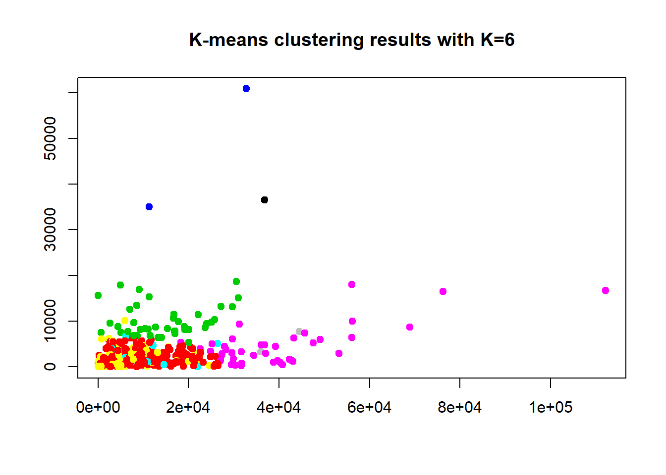
plot(df[c("Fresh", "Milk")], col=km.out1$cluster)
points(km.out1$centers[,c("Fresh", "Milk")], pch=1, cex=3, col="red", lwd=2)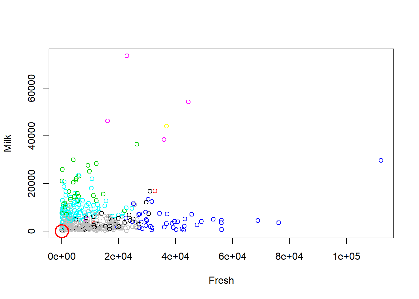
plot(df[c("Fresh", "Frozen")], col=km.out1$cluster)
points(km.out1$centers[,c("Fresh", "Frozen")], pch=1, cex=3, col="red", lwd=2)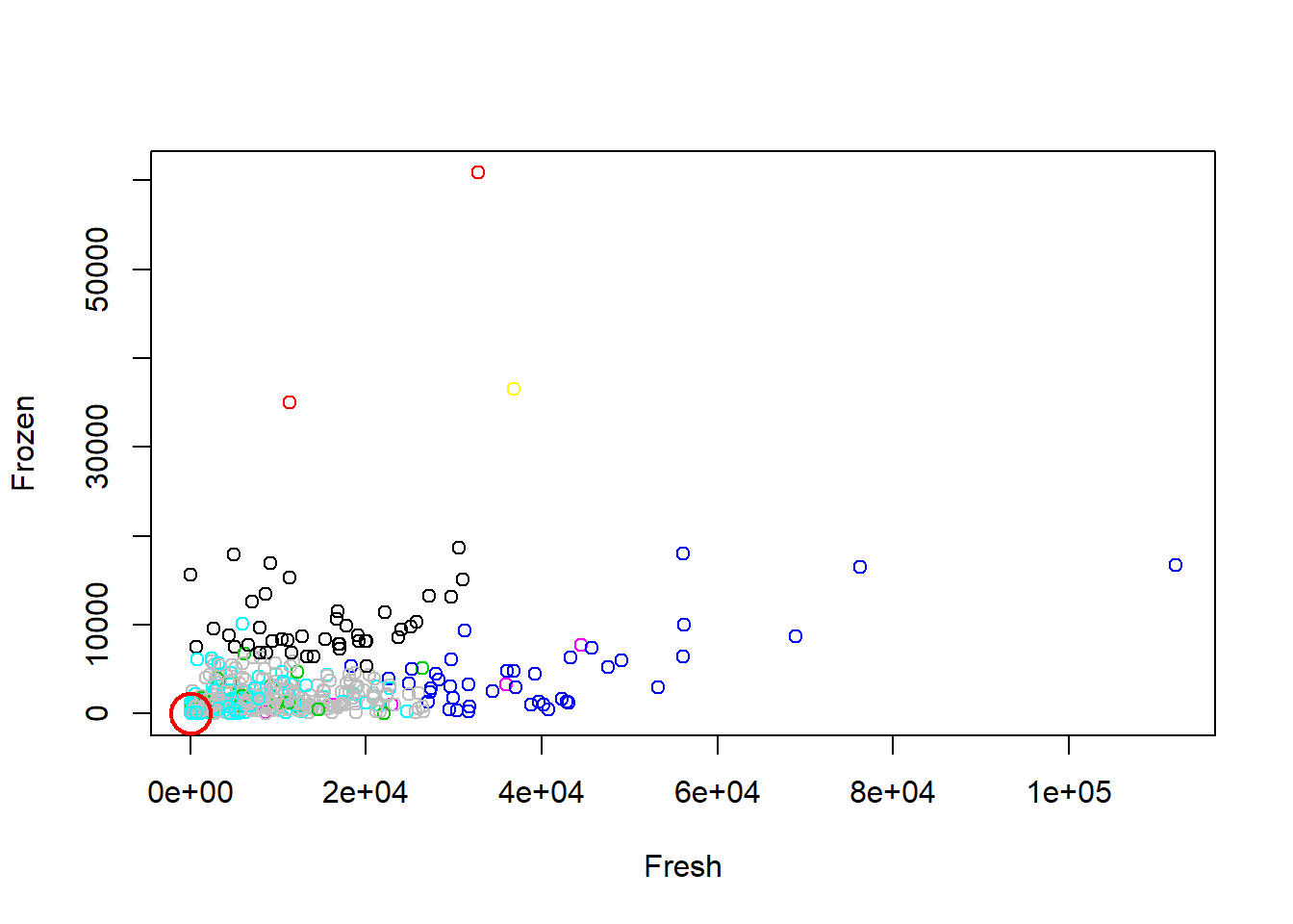
Here we run the full scaled data and check 2 to 10 clusters for the best option. The graph is clear with a steady decline down from 2. the WCSS decreases. The elbow of the silhouette width plot is interesting because it drops after 2 clusters but bounces back up to 4 before dropping again. This unknown why it does this but we are still in the 2 cluster option. But this test is telling us 4 clusters is the optimal value. If it says 4 then we will run the k=4 and produce a WCSS 47.8% which doesn’t seem better that 2 clusters at 26% WCSS. The center of the points show 3 in the bottom left which is expected and one up in the top left which is completely unexpected and confusing. Something doesn’t seem right here and it is unknown what that is.
nk <- 2:10
set.seed(22)
WSS <- sapply(nk, function(k) {kmeans(df_z, centers = k)$tot.withinss})
WSS
## [1] 2593.4767 2269.5053 1944.3840 1676.5956 1467.4379 1186.9108 1120.7044
## [8] 1031.2988 908.9784plot(nk, WSS, type="l", xlab="number of k", ylab="within sum of squares")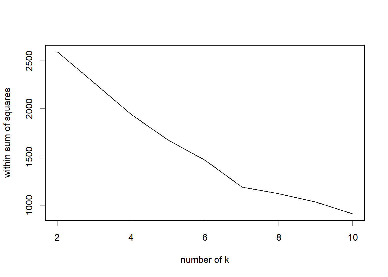
SW <- sapply(nk, function(k) {cluster.stats(dist(df_z), kmeans(df_z,centers=k)$cluster)$avg.silwidth})
SW
## [1] 0.3732334 0.3067572 0.3224285 0.3562636 0.3469665 0.2809717 0.3482999
## [8] 0.3277299 0.3257194plot(nk, SW, type="l", xlab="number ofclusters", ylab="average silhouette width")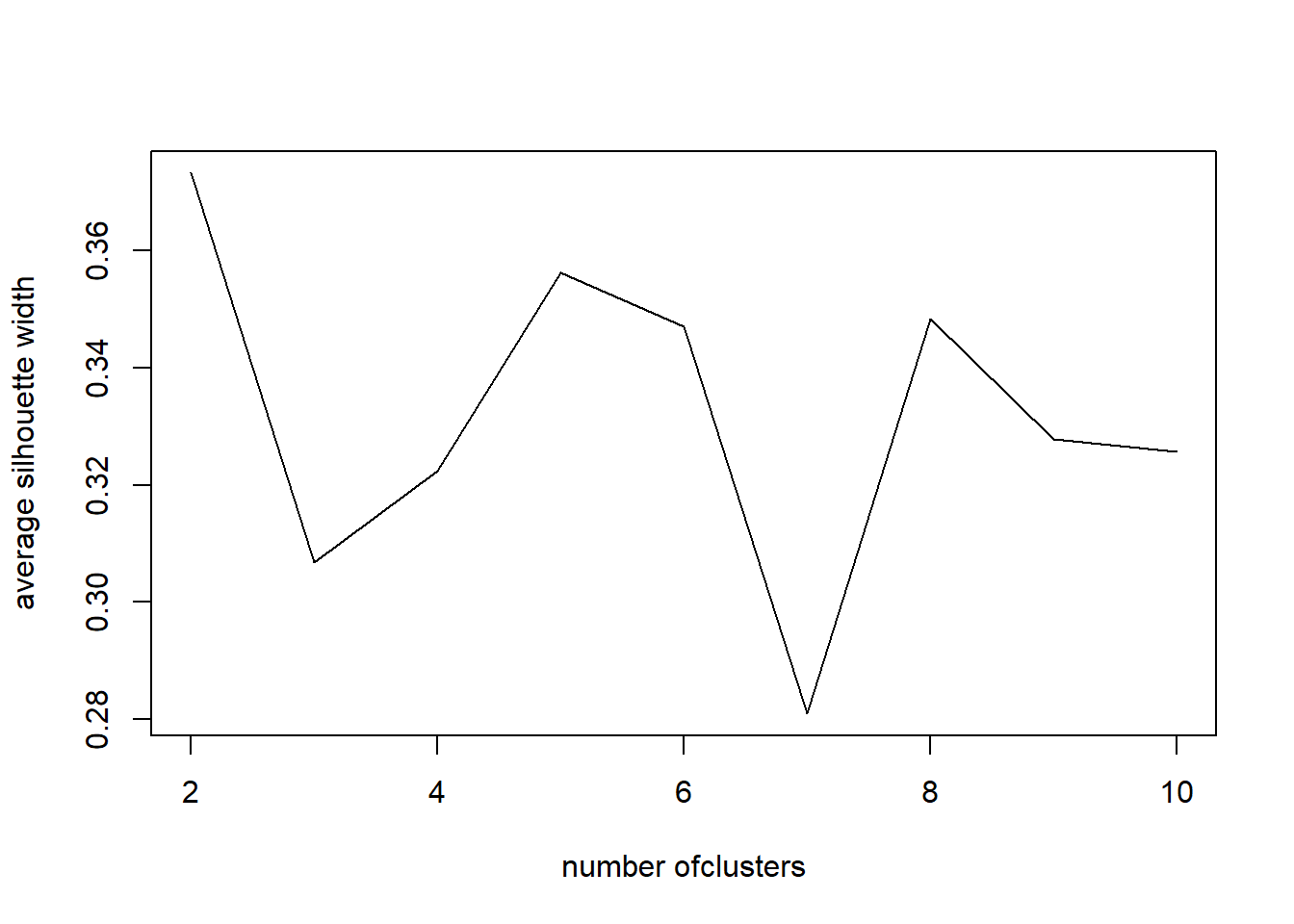
nk[which.max(SW)]## [1] 2km.out <- kmeans(df_z, 4, nstart = 20)
km.out## K-means clustering with 4 clusters of sizes 10, 296, 3, 131
##
## Cluster means:
## Channel Region Fresh Milk Grocery Frozen
## 1 1.4470045 -0.05577083 0.31347349 3.9174467 4.2707490 -0.003570131
## 2 -0.6822942 -0.04704424 0.07979916 -0.3554503 -0.4344436 0.073138067
## 3 -0.6895122 0.15948501 3.84044484 3.2957757 0.9852919 7.204892918
## 4 1.4470045 0.10690343 -0.29218794 0.4286373 0.6330682 -0.329983553
## Detergents_Paper Delicassen
## 1 4.6129149 0.50279301
## 2 -0.4417690 -0.10544775
## 3 -0.1527927 6.79967230
## 4 0.6495639 0.04416479
##
## Clustering vector:
## [1] 4 4 4 2 4 4 4 4 2 4 4 4 4 4 4 2 4 2 4 2 4 2 2 4 4 4 2 2 4 2 2 2 2 2 2 4 2
## [38] 4 4 2 2 2 4 4 4 4 4 1 4 4 2 2 4 4 2 2 1 4 2 2 4 1 4 4 2 1 2 4 2 2 2 2 2 4
## [75] 4 2 2 4 2 2 2 4 4 2 4 1 1 2 2 2 2 2 1 2 4 2 4 2 2 2 4 4 4 2 2 2 4 4 4 4 2
## [112] 4 2 2 2 2 2 2 2 2 2 2 2 4 2 2 2 4 2 2 2 2 2 2 2 2 2 2 2 2 2 2 2 2 2 4 2 2
## [149] 2 2 2 2 2 2 2 4 4 2 4 4 4 2 2 4 4 4 4 2 2 2 4 4 2 4 2 4 2 2 2 2 2 3 2 3 2
## [186] 2 2 2 4 4 2 2 2 4 2 2 2 4 2 2 4 4 2 2 2 4 2 4 2 4 2 1 2 2 4 2 4 2 4 2 2 2
## [223] 2 4 2 2 4 2 2 2 4 2 2 2 2 2 2 2 2 2 2 2 2 2 2 4 2 2 2 2 2 1 2 2 2 2 2 2 2
## [260] 2 2 2 2 2 4 2 4 2 4 2 2 2 2 2 2 2 2 2 2 4 2 4 2 2 2 2 2 2 2 2 2 2 2 4 2 4
## [297] 2 4 4 2 4 4 4 4 4 4 4 2 2 4 2 2 4 2 2 4 2 2 2 4 2 2 2 2 2 3 2 2 2 2 2 4 2
## [334] 1 2 4 2 2 2 2 4 4 2 4 2 2 4 4 2 4 2 4 2 4 2 2 2 4 2 2 2 2 2 2 2 4 2 2 2 2
## [371] 4 2 2 4 2 2 4 2 2 4 2 2 2 2 2 2 2 2 2 2 2 2 2 2 2 2 4 2 2 2 2 2 2 2 2 2 2
## [408] 4 4 2 2 2 2 2 2 4 4 2 4 2 2 4 2 4 4 2 2 2 2 2 2 2 2 2 2 2 2 4 2 2
##
## Within cluster sum of squares by cluster:
## [1] 160.2905 1020.2318 215.6517 437.3645
## (between_SS / total_SS = 47.8 %)
##
## Available components:
##
## [1] "cluster" "centers" "totss" "withinss" "tot.withinss"
## [6] "betweenss" "size" "iter" "ifault"plot(df_z$Fresh, col=(km.out$cluster+2), main="K-means clustering results with K=4", xlab="", ylab="", pch=19, cex=0.7)
points(km.out$centers[,c("Fresh", "Frozen")], pch=1, cex=3, col="red", lwd=2)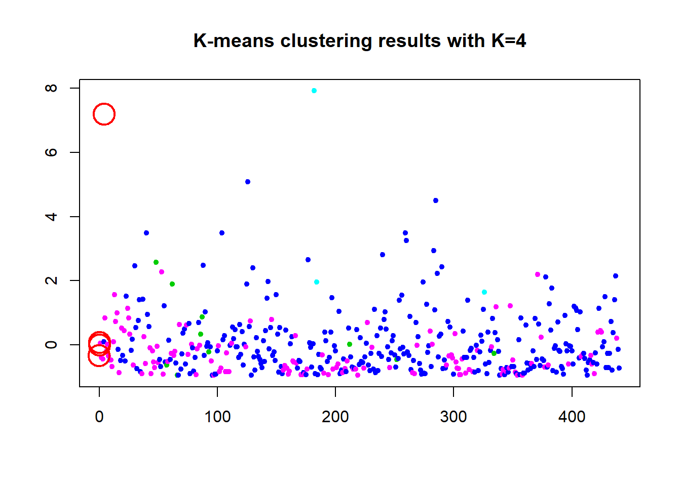
Hierarchial Cluster Analysis
This exercise produces a mess of a dendrograph but the general shape of how it breaks down the data is somewhat legible by shapes only. Complete linkage seems the best. Single linkage is very hard to read.
set.seed(89)
km <- kmeans(df_z, 4, nstart = 20)
hc.complete <- hclust(dist(df_z), method= "complete")
hc.average <-  hclust(dist(df_z), method= "average")
hc.single <- hclust(dist(df_z), method= "single")
#Bad display par(mfrow =c(1,3))
plot(hc.complete, main="Complete Linkage", xlab ="", sub ="", cex =0.05)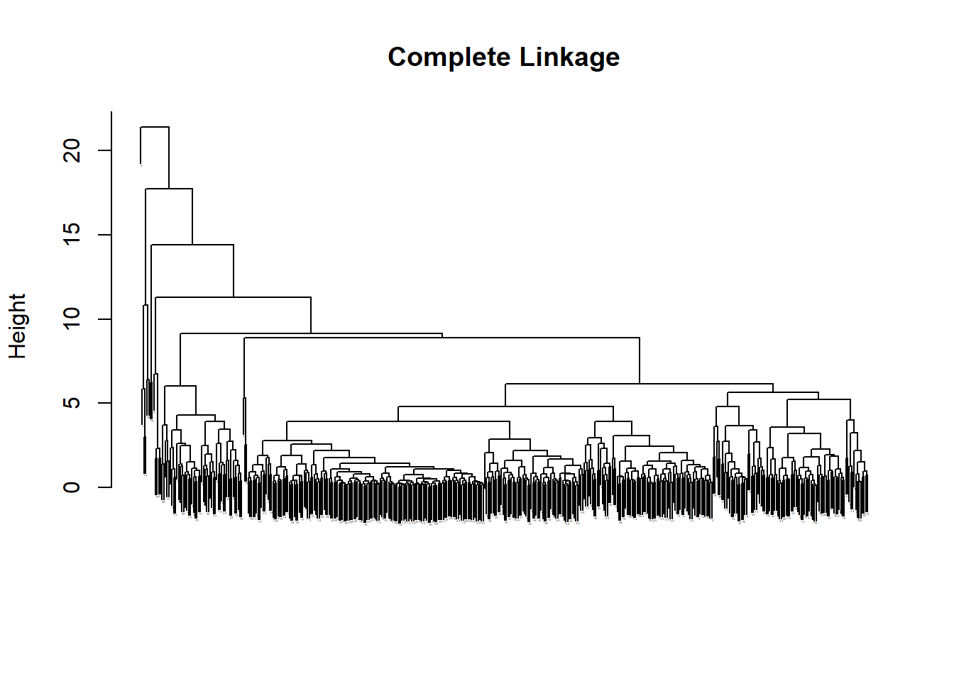
plot(hc.average, main="Average Linkage", xlab ="", sub ="", cex =0.05)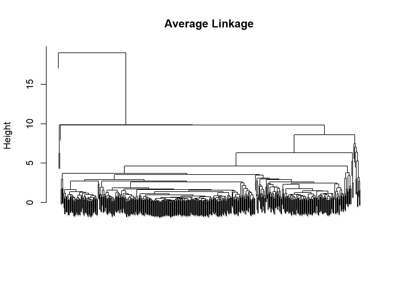
plot(hc.single, main="Single Linkage", xlab ="", sub ="", cex =0.01)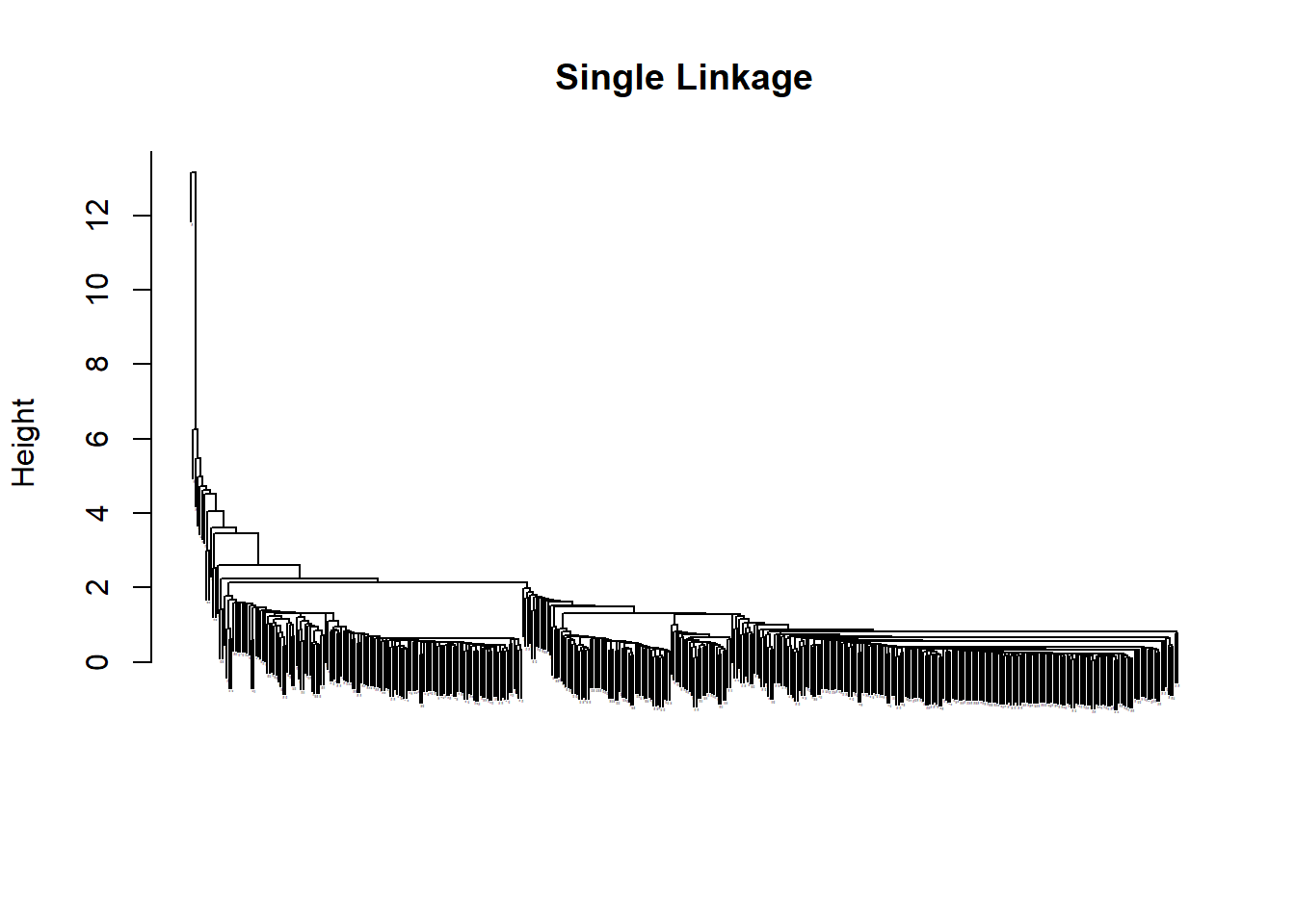
##   [1] 1 1 1 1 1 1 1 1 1 1 1 1 1 1 1 1 1 1 1 1 1 1 1 1 1 1 1 1 1 1 1 1 1 1 1 1 1
##  [38] 1 1 1 1 1 1 1 1 1 1 1 1 1 1 1 1 1 1 1 1 1 1 1 1 1 1 1 1 1 1 1 1 1 1 1 1 1
##  [75] 1 1 1 1 1 1 1 1 1 1 1 1 1 1 1 1 1 1 1 1 1 1 1 1 1 1 1 1 1 1 1 1 1 1 1 1 1
## [112] 1 1 1 1 1 1 1 1 1 1 1 1 1 1 1 1 1 1 1 1 1 1 1 1 1 1 1 1 1 1 1 1 1 1 1 1 1
## [149] 1 1 1 1 1 1 1 1 1 1 1 1 1 1 1 1 1 1 1 1 1 1 1 1 1 1 1 1 1 1 1 1 1 1 1 2 1
## [186] 1 1 1 1 1 1 1 1 1 1 1 1 1 1 1 1 1 1 1 1 1 1 1 1 1 1 1 1 1 1 1 1 1 1 1 1 1
## [223] 1 1 1 1 1 1 1 1 1 1 1 1 1 1 1 1 1 1 1 1 1 1 1 1 1 1 1 1 1 1 1 1 1 1 1 1 1
## [260] 1 1 1 1 1 1 1 1 1 1 1 1 1 1 1 1 1 1 1 1 1 1 1 1 1 1 1 1 1 1 1 1 1 1 1 1 1
## [297] 1 1 1 1 1 1 1 1 1 1 1 1 1 1 1 1 1 1 1 1 1 1 1 1 1 1 1 1 1 1 1 1 1 1 1 1 1
## [334] 1 1 1 1 1 1 1 1 1 1 1 1 1 1 1 1 1 1 1 1 1 1 1 1 1 1 1 1 1 1 1 1 1 1 1 1 1
## [371] 1 1 1 1 1 1 1 1 1 1 1 1 1 1 1 1 1 1 1 1 1 1 1 1 1 1 1 1 1 1 1 1 1 1 1 1 1
## [408] 1 1 1 1 1 1 1 1 1 1 1 1 1 1 1 1 1 1 1 1 1 1 1 1 1 1 1 1 1 1 1 1 1
## [1] 1 1 1 1 1 1 1 1 1 1 1 1 1 1 1 1 1 1 1 1 1 1 1 1 1 1 1 1 1 1 1 1 1 1 1 1 1
## [38] 1 1 1 1 1 1 1 1 1 1 1 1 1 1 1 1 1 1 1 1 1 1 1 1 1 1 1 1 1 1 1 1 1 1 1 1 1
## [75] 1 1 1 1 1 1 1 1 1 1 1 1 1 1 1 1 1 1 1 1 1 1 1 1 1 1 1 1 1 1 1 1 1 1 1 1 1
## [112] 1 1 1 1 1 1 1 1 1 1 1 1 1 1 1 1 1 1 1 1 1 1 1 1 1 1 1 1 1 1 1 1 1 1 1 1 1
## [149] 1 1 1 1 1 1 1 1 1 1 1 1 1 1 1 1 1 1 1 1 1 1 1 1 1 1 1 1 1 1 1 1 1 1 1 2 1
## [186] 1 1 1 1 1 1 1 1 1 1 1 1 1 1 1 1 1 1 1 1 1 1 1 1 1 1 1 1 1 1 1 1 1 1 1 1 1
## [223] 1 1 1 1 1 1 1 1 1 1 1 1 1 1 1 1 1 1 1 1 1 1 1 1 1 1 1 1 1 1 1 1 1 1 1 1 1
## [260] 1 1 1 1 1 1 1 1 1 1 1 1 1 1 1 1 1 1 1 1 1 1 1 1 1 1 1 1 1 1 1 1 1 1 1 1 1
## [297] 1 1 1 1 1 1 1 1 1 1 1 1 1 1 1 1 1 1 1 1 1 1 1 1 1 1 1 1 1 1 1 1 1 1 1 1 1
## [334] 1 1 1 1 1 1 1 1 1 1 1 1 1 1 1 1 1 1 1 1 1 1 1 1 1 1 1 1 1 1 1 1 1 1 1 1 1
## [371] 1 1 1 1 1 1 1 1 1 1 1 1 1 1 1 1 1 1 1 1 1 1 1 1 1 1 1 1 1 1 1 1 1 1 1 1 1
## [408] 1 1 1 1 1 1 1 1 1 1 1 1 1 1 1 1 1 1 1 1 1 1 1 1 1 1 1 1 1 1 1 1 1## [1] 1 1 1 1 1 1 1 1 1 1 1 1 1 1 1 1 1 1 1 1 1 1 1 1 1 1 1 1 1 1 1 1 1 1 1 1 1
## [38] 1 1 1 1 1 1 1 1 1 1 1 1 1 1 1 1 1 1 1 1 1 1 1 1 1 1 1 1 1 1 1 1 1 1 1 1 1
## [75] 1 1 1 1 1 1 1 1 1 1 1 1 1 1 1 1 1 1 1 1 1 1 1 1 1 1 1 1 1 1 1 1 1 1 1 1 1
## [112] 1 1 1 1 1 1 1 1 1 1 1 1 1 1 1 1 1 1 1 1 1 1 1 1 1 1 1 1 1 1 1 1 1 1 1 1 1
## [149] 1 1 1 1 1 1 1 1 1 1 1 1 1 1 1 1 1 1 1 1 1 1 1 1 1 1 1 1 1 1 1 1 1 2 1 3 1
## [186] 1 1 1 1 1 1 1 1 1 1 1 1 1 1 1 1 1 1 1 1 1 1 1 1 1 1 1 1 1 1 1 1 1 1 1 1 1
## [223] 1 1 1 1 1 1 1 1 1 1 1 1 1 1 1 1 1 1 1 1 1 1 1 1 1 1 1 1 1 1 1 1 1 1 1 1 1
## [260] 1 1 1 1 1 1 1 1 1 1 1 1 1 1 1 1 1 1 1 1 1 1 1 1 1 1 1 1 1 1 1 1 1 1 1 1 1
## [297] 1 1 1 1 1 1 1 1 1 1 1 1 1 1 1 1 1 1 1 1 1 1 1 1 1 1 1 1 1 4 1 1 1 1 1 1 1
## [334] 1 1 1 1 1 1 1 1 1 1 1 1 1 1 1 1 1 1 1 1 1 1 1 1 1 1 1 1 1 1 1 1 1 1 1 1 1
## [371] 1 1 1 1 1 1 1 1 1 1 1 1 1 1 1 1 1 1 1 1 1 1 1 1 1 1 1 1 1 1 1 1 1 1 1 1 1
## [408] 1 1 1 1 1 1 1 1 1 1 1 1 1 1 1 1 1 1 1 1 1 1 1 1 1 1 1 1 1 1 1 1 1xsc <- scale(df_z)plot(hclust(dist(xsc), method= "complete"), main= "Hierarchical Clustering with Scaled Features", cex =0.01)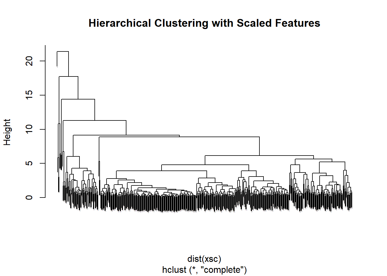
This graph uses complete linkage and produces a legible dendogram. The WCSS is 1846 and average silwidth of 0.34. Comparatively, the single to complete give 2918 and 3159 WCSS and ASW 0.66 and 0.82. Is this good? More descriptive direction is needed on this output. I guess its good?
x <- matrix(rnorm (30*3), ncol =3)
dd <- as.dist(1-cor(t(x)))
plot(hclust(dd, method= "complete"), main= "Complete Linkage with Correlation - Based Distance", xlab="", sub="")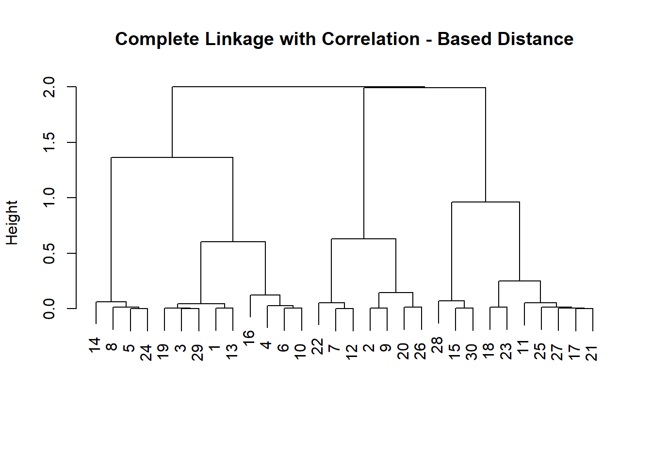
hc_complete <- cutree(hc.complete, 2)
hc_single <- cutree(hc.single, 4)
#library fpc
cs <- cluster.stats(dist(df_z), km$cluster)
cs[c("within.cluster.ss", "avg.silwidth")]
## $within.cluster.ss
## [1] 1833.538
##
## $avg.silwidth
## [1] 0.3674071sapply(list(kmeans=km$cluster, hc_single=hc_single, hc_complete=hc_complete), function(c) cluster.stats(dist(df_z), c)[c("within.cluster.ss", "avg.silwidth")])## kmeans hc_single hc_complete
## within.cluster.ss 1833.538 2918.012 3159.398
## avg.silwidth 0.3674071 0.6678067 0.8263512This method is an alternate to the one above. Maybe better graphing and understanding of what is happening can be gained from this method. The first part determines the optimal number of clusters. We will also drop the Channel and Region variables for this section. This method is straight forward and clearly shows 9 proposed as 2 is the best number of clusters. The data spells it out and the bar chart clearly shows us 2 clusters is optimal with a 3 the next optimal.
Optional Alternative Method
df_hc <- df_z[3:8]
str(df_hc)
## 'data.frame': 440 obs. of 6 variables:
## $ Fresh : num 0.0529 -0.3909 -0.4465 0.1 0.8393 ...
## $ Milk : num 0.523 0.5438 0.4081 -0.6233 -0.0523 ...
## $ Grocery : num -0.0411 0.1701 -0.0281 -0.3925 -0.0793 ...
## $ Frozen : num -0.589 -0.27 -0.137 0.686 0.174 ...
## $ Detergents_Paper: num -0.0435 0.0863 0.1331 -0.498 -0.2317 ...
## $ Delicassen : num -0.0663 0.089 2.2407 0.0933 1.2979 ...nb <- NbClust(df_hc, distance="euclidean", min.nc = 2, max.nc = 10, method = "complete", index = "all")## Warning in pf(beale, pp, df2): NaNs produced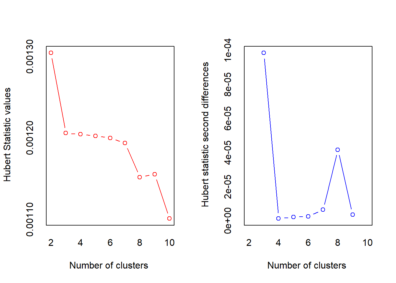
## *** : The Hubert index is a graphical method of determining the number of clusters.
##                 In the plot of Hubert index, we seek a significant knee that corresponds to a
##                 significant increase of the value of the measure i.e the significant peak in Hubert
##                 index second differences plot.
## 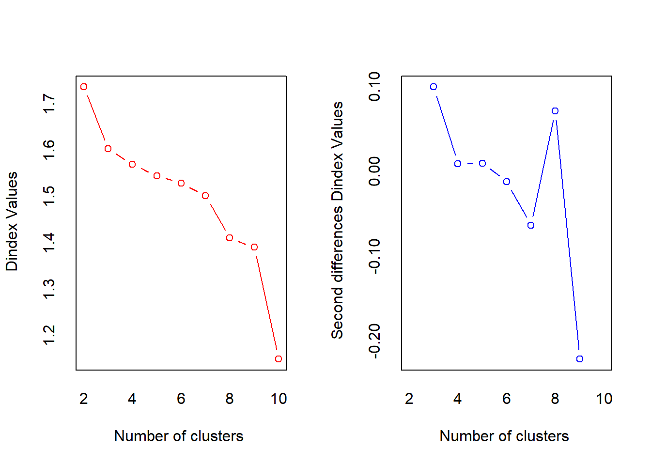
## *** : The D index is a graphical method of determining the number of clusters.
##                 In the plot of D index, we seek a significant knee (the significant peak in Dindex
##                 second differences plot) that corresponds to a significant increase of the value of
##                 the measure.
##
## *******************************************************************
## * Among all indices:
## * 9 proposed 2 as the best number of clusters
## * 7 proposed 3 as the best number of clusters
## * 1 proposed 4 as the best number of clusters
## * 1 proposed 7 as the best number of clusters
## * 2 proposed 8 as the best number of clusters
## * 4 proposed 10 as the best number of clusters
##
##                    ***** Conclusion *****
##
## * According to the majority rule, the best number of clusters is  2
##
##
## *******************************************************************
fviz_nbclust(nb) + theme_minimal()## Among all indices:
## ===================
## * 2 proposed 0 as the best number of clusters
## * 9 proposed 2 as the best number of clusters
## * 7 proposed 3 as the best number of clusters
## * 1 proposed 4 as the best number of clusters
## * 1 proposed 7 as the best number of clusters
## * 2 proposed 8 as the best number of clusters
## * 4 proposed 10 as the best number of clusters
##
## Conclusion
## =========================
## * According to the majority rule, the best number of clusters is 2 .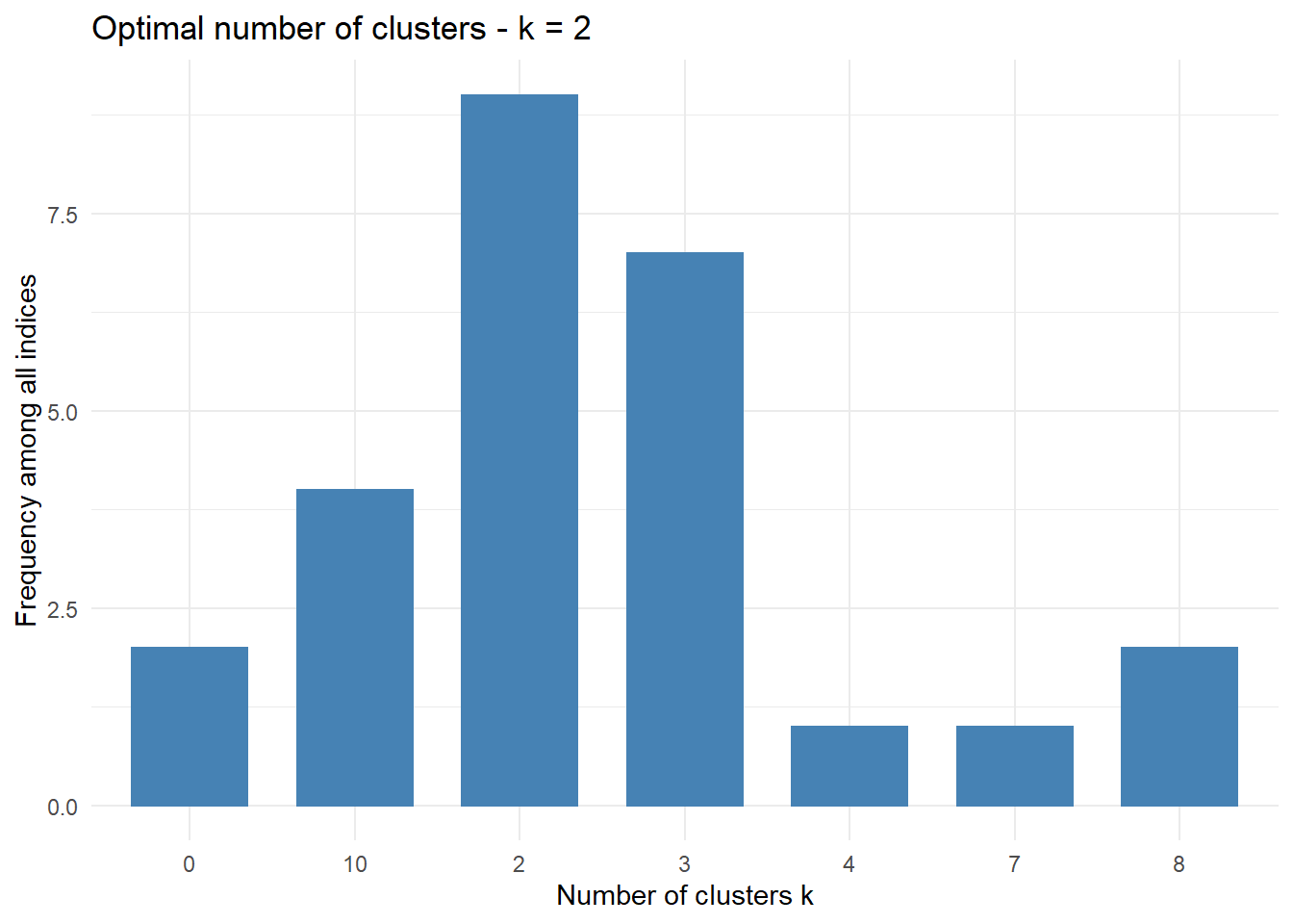
km.res <- eclust(df_hc, "kmeans", k = 2, nstart=25, graph = FALSE)
km.res$cluster
## [1] 2 2 2 2 2 2 2 2 2 2 2 2 2 2 2 2 2 2 2 2 2 2 2 1 2 2 2 2 1 2 2 2 2 2 2 2 2
## [38] 2 2 2 2 2 2 1 2 1 1 1 2 1 2 2 2 2 2 2 1 2 2 2 2 1 2 2 2 1 2 2 2 2 2 2 2 2
## [75] 2 2 2 1 2 2 2 2 2 2 2 1 1 2 2 2 2 2 1 2 2 2 2 2 2 2 2 2 2 2 2 2 2 2 2 2 2
## [112] 2 2 2 2 2 2 2 2 2 2 2 2 2 2 2 2 2 2 2 2 2 2 2 2 2 2 2 2 2 2 2 2 2 2 1 2 2
## [149] 2 2 2 2 2 2 2 1 2 2 2 2 2 2 2 1 2 1 2 2 2 2 2 1 2 2 2 2 2 2 2 2 2 1 2 1 2
## [186] 2 2 2 2 2 2 2 2 2 2 2 2 2 2 2 1 1 2 2 2 1 2 2 2 1 2 1 2 2 2 2 1 2 2 2 2 2
## [223] 2 2 2 2 2 2 2 2 2 2 2 2 2 2 2 2 2 2 2 2 2 2 2 2 2 2 2 2 2 1 2 2 2 2 2 2 2
## [260] 2 2 2 2 2 2 2 2 2 2 2 2 2 2 2 2 2 2 2 2 2 2 2 2 2 2 2 2 2 2 2 2 2 2 2 2 2
## [297] 2 2 2 2 2 1 2 2 1 2 1 2 2 1 2 2 1 2 2 2 2 2 2 1 2 2 2 2 2 1 2 2 2 2 2 1 2
## [334] 1 2 2 2 2 2 2 2 2 2 1 2 2 2 2 2 1 2 1 2 2 2 2 2 2 2 2 2 2 2 2 2 2 2 2 2 2
## [371] 2 2 2 2 2 2 2 2 2 2 2 2 2 2 2 2 2 2 2 2 2 2 2 2 2 2 2 2 2 2 2 2 2 2 2 2 2
## [408] 2 2 2 2 2 2 2 2 2 2 2 2 2 2 2 2 2 2 2 2 2 2 2 2 2 2 2 2 2 2 1 2 2The cluster plot is now more legible in this graphic. k=2 and the center of cluster 1 is a red dot and the center of cluster 2 is the blue triangle.
fviz_cluster(km.res, geom="point", ellipse.type="norm")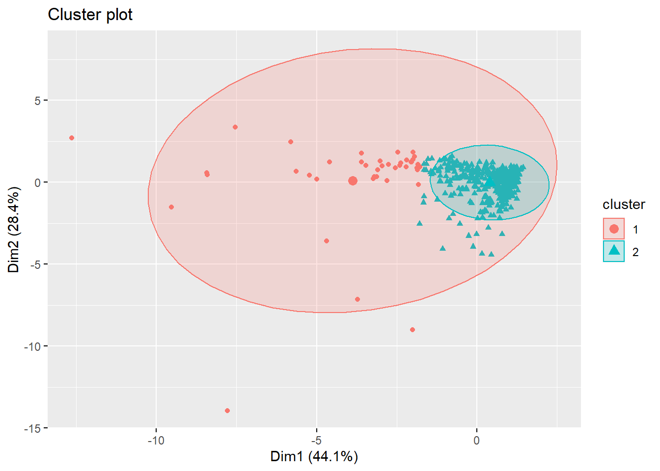
pam.res <- eclust(df_hc, "pam", k=2, graph=FALSE)
pam.res$cluster
## [1] 1 2 2 1 1 1 1 1 1 2 2 1 2 2 2 1 2 1 1 1 1 1 1 2 2 1 1 1 2 1 1 1 1 1 1 1 1
## [38] 2 2 1 1 1 2 2 1 2 2 2 2 2 1 1 1 2 1 1 2 2 1 1 1 2 1 2 1 2 1 2 1 1 1 2 1 1
## [75] 1 1 1 2 1 1 1 2 2 1 1 2 2 1 1 1 1 1 2 1 2 1 1 1 1 1 2 2 1 1 1 1 2 2 1 2 1
## [112] 2 1 1 1 1 1 1 1 1 1 1 1 1 1 1 1 1 1 1 1 1 1 1 1 1 1 1 1 1 1 1 1 1 1 2 1 1
## [149] 1 1 1 1 1 1 1 2 2 1 1 2 2 1 1 2 1 2 2 1 1 1 2 2 1 2 1 2 1 1 1 1 1 2 2 2 1
## [186] 1 1 1 2 2 1 1 1 2 1 1 1 2 1 1 2 2 1 1 1 2 1 1 1 2 1 2 1 1 2 2 2 1 2 1 1 2
## [223] 1 1 1 1 1 1 1 1 1 1 1 1 1 1 1 1 1 1 1 1 1 1 1 2 1 1 1 1 1 2 1 1 2 1 1 1 1
## [260] 1 1 1 1 1 2 2 2 1 2 1 1 1 1 1 1 1 1 1 1 1 1 1 1 1 1 1 1 1 1 1 1 1 1 2 1 1
## [297] 1 1 1 1 1 2 2 2 2 2 2 1 1 2 1 1 2 1 1 2 1 1 1 2 1 1 1 1 1 1 1 1 1 1 1 2 1
## [334] 2 1 1 1 1 1 1 2 2 1 2 1 1 2 1 1 2 1 2 1 2 1 1 1 2 1 1 1 1 1 1 1 1 1 1 1 1
## [371] 1 1 1 1 1 1 2 1 1 1 1 1 1 1 2 1 1 1 1 1 1 1 1 1 1 1 2 1 1 1 1 1 1 1 1 1 1
## [408] 2 1 1 1 1 1 1 1 1 2 1 2 1 2 1 1 1 1 1 2 1 1 1 1 1 1 1 1 1 1 2 1 1fviz_cluster(pam.res, geom="point", ellipse.type="norm")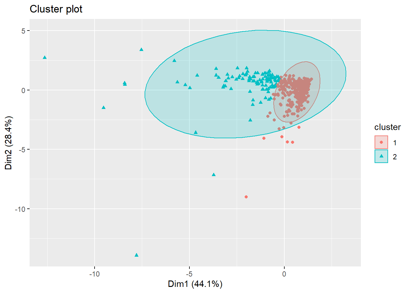
res.hc <- eclust(df_hc, "hclust", k=2, method="complete", graph=FALSE)
head(res.hc$cluster, 10)
## [1] 1 1 1 1 1 1 1 1 1 1This dendogram is better than before with some color added. However the cluster 1 is stuffed in the left corner.
fviz_dend(res.hc, rect=TRUE, show_labels=FALSE)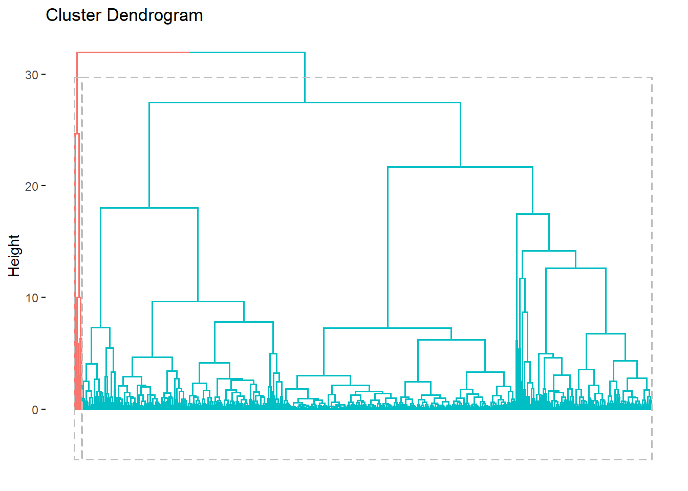
sil <- silhouette(km.res$cluster, dist(df_hc))
head(sil[,1:3], 10)
## cluster neighbor sil_width
## [1,] 2 1 0.6614836
## [2,] 2 1 0.6378712
## [3,] 2 1 0.4547508
## [4,] 2 1 0.7168852
## [5,] 2 1 0.5961813
## [6,] 2 1 0.7059518
## [7,] 2 1 0.7204588
## [8,] 2 1 0.6808825
## [9,] 2 1 0.7349506
## [10,] 2 1 0.3320876fviz_silhouette(sil)## cluster size ave.sil.width
## 1 1 41 0.03
## 2 2 399 0.65
si.sum <- summary(sil)
si.sum$clus.avg.widths
## 1 2
## 0.02503374 0.64967036si.sum$avg.width## [1] 0.5914656si.sum$clus.sizes## cl
## 1 2
## 41 399fviz_silhouette(km.res)## cluster size ave.sil.width
## 1 1 41 0.03
## 2 2 399 0.65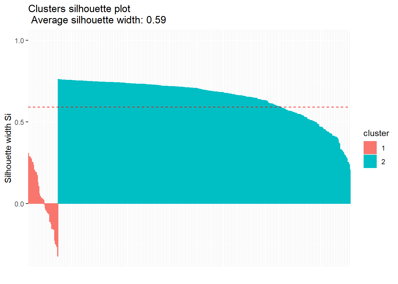
silinfo <- km.res$silinfonames(silinfo)## [1] "widths" "clus.avg.widths" "avg.width"head(silinfo$widths)## cluster neighbor sil_width
## 212 1 2 0.3089443
## 93 1 2 0.2887751
## 66 1 2 0.2857945
## 62 1 2 0.2785948
## 252 1 2 0.2713289
## 57 1 2 0.2534072silinfo$clus.avg.widths## [1] 0.02503374 0.64967036silinfo$avg.width## [1] 0.5914656km.res$size## [1] 41 399dd <- dist(df_hc, method = "euclidean")
km_stats <- cluster.stats(dd, km.res$cluster)
km_stats$within.cluster.ss## [1] 1949.348km_stats$clus.avg.silwidths## 1 2
## 0.02503374 0.64967036The Dunn statistic is 0.0189 and Dunn2 1.07.
km_stats## $n
## [1] 440
##
## $cluster.number
## [1] 2
##
## $cluster.size
## [1] 41 399
##
## $min.cluster.size
## [1] 41
##
## $noisen
## [1] 0
##
## $diameter
## [1] 21.244265 7.938436
##
## $average.distance
## [1] 5.223323 1.933809
##
## $median.distance
## [1] 3.149260 1.726398
##
## $separation
## [1] 0.4019017 0.4019017
##
## $average.toother
## [1] 5.595136 5.595136
##
## $separation.matrix
## [,1] [,2]
## [1,] 0.0000000 0.4019017
## [2,] 0.4019017 0.0000000
##
## $ave.between.matrix
## [,1] [,2]
## [1,] 0.000000 5.595136
## [2,] 5.595136 0.000000
##
## $average.between
## [1] 5.595136
##
## $average.within
## [1] 2.240332
##
## $n.between
## [1] 16359
##
## $n.within
## [1] 80221
##
## $max.diameter
## [1] 21.24427
##
## $min.separation
## [1] 0.4019017
##
## $within.cluster.ss
## [1] 1949.348
##
## $clus.avg.silwidths
##          1          2
## 0.02503374 0.64967036
##
## $avg.silwidth
## [1] 0.5914656
##
## $g2
## NULL
##
## $g3
## NULL
##
## $pearsongamma
## [1] 0.5891823
##
## $dunn
## [1] 0.01891813
##
## $dunn2
## [1] 1.071183
##
## $entropy
## [1] 0.3098382
##
## $wb.ratio
## [1] 0.400407
##
## $ch
## [1] 153.8348
##
## $cwidegap
## [1] 12.977504 3.612317
##
## $widestgap
## [1] 12.9775
##
## $sindex
## [1] 0.9162984
##
## $corrected.rand
## NULL
##
## $vi
## NULL