Reinforcement Learning - Grid World Problem
The first section looks at the grid world concept/problem. The environment is a 3x4 grid and the goal is to move from the start xy (1,1) (called a “state”") location to the opposite corner (4,3) called the goal state. The actions are up, down, left, right. We have the rewards of +1 & -1. We want the agent to find the shortest sequence of actions to get from start to end (goal). The additional rules are blocking the the state labeled by x=2/y=2 and avoiding the forfeiture state of x=4/y=2. Thus from the start state we can only go up or right. This is a delayed reward state concept because several moves need to be made before getting to the goal state.
#state, action, rewards, and policy concepts using Grid World concept.
#actions: up, down, left , right
#rewards: +1, -1
#find the shortest sequence of actions to get to the goal
actions <- c("U", "D", "L", "R")
actions
## [1] "U" "D" "L" "R"#construct the environment
x <- 1:4 #four rows
x## [1] 1 2 3 4y <- 1:3 #three columns
y## [1] 1 2 3# construct the states
states <- expand.grid(x=x, y=y)
states## x y
## 1 1 1
## 2 2 1
## 3 3 1
## 4 4 1
## 5 1 2
## 6 2 2
## 7 3 2
## 8 4 2
## 9 1 3
## 10 2 3
## 11 3 3
## 12 4 3#construct the reward matrix
rewards <- matrix(rep(0, 12), nrow=3) #3X4 matrix start with 0 values
rewards## [,1] [,2] [,3] [,4]
## [1,] 0 0 0 0
## [2,] 0 0 0 0
## [3,] 0 0 0 0rewards[2,2] <-NA
rewards## [,1] [,2] [,3] [,4]
## [1,] 0 0 0 0
## [2,] 0 NA 0 0
## [3,] 0 0 0 0rewards[1,4] <- 1 #goal state reward of 1
rewards[2,4] <- -1 #forefiture state of -1
#Absorbing rewardsHere is a method to finish the game quickly by adding a small negative reward of -0.04 verses 0. Note the matrix replaced all the 0’s with -0.04.
rewards <- matrix(rep(-0.04, 12), nrow=3) #modify to finish game quickly as possible by adding -0.04
rewards[2,2] <- NA
rewards[1,4] <- 1
rewards[2,4] <- -1
rewards #3 X 4 reward matrix note 1 at (4,1)= goal state
## [,1] [,2] [,3] [,4]
## [1,] -0.04 -0.04 -0.04 1.00
## [2,] -0.04 NA -0.04 -1.00
## [3,] -0.04 -0.04 -0.04 -0.04The transition probability introduces some notion of uncertainty as to what is the actual action that is implemented when we try to take and action. There is some randomness involved where the action moves. Below we build in the randomness with probability of which direction the agent will move.
#transition probabilities 80% and 10% probability
transition <- list("U" = c("U"=0.8, "D"=0, "L"=0.1, "R"=0.1),
                   "D" = c("D"=0.8, "U"=0, "L"=0.1, "R"=0.1),
                   "L" = c("L"=0.8, "R"=0, "U"=0.1, "D" =0.1),
                   "R" = c("R"=0.8, "L"=0, "U"=0.1, "D" =0.1))
transition
## $U
## U D L R
## 0.8 0.0 0.1 0.1
##
## $D
## D U L R
## 0.8 0.0 0.1 0.1
##
## $L
## L R U D
## 0.8 0.0 0.1 0.1
##
## $R
## R L U D
## 0.8 0.0 0.1 0.1#action value 1 increases x,Y -1 decreases X,Y. Incrementing the values of x,y to show action values.
action.values <- list ("U" = c("X" =0, "Y" =1),
"D" = c("X" =0, "Y" =-1),
"L" = c("X" =-1, "Y" =0),
"R" = c("X" =1, "Y" =0))
action.values## $U
## X Y
## 0 1
##
## $D
## X Y
## 0 -1
##
## $L
## X Y
## -1 0
##
## $R
## X Y
## 1 0The best policy is up, up, right, right, right to the goal “1”. Below we get into the reinforcement learning package with an example navigating a 2X2 grid. The agent interacts with the environment and takes actions that effect the state of the environment. There is limited rewards that tell the agent its performance and the goal is to improve behavior with limited rewards. There are only 4 states in this example and a rule set that the action can not be made from x=1/y=1 over to x=2/y=2 (goal) state. The s1,s2,s3 are 1 and goal s4 is 10 reward points. The actions are up, down, left, right. The gridworldEnvironment comes with the package and defines this 2x2 gridworld.
#########################
#State-Action-Reward with policy iteration
library(ReinforcementLearning)
#2x2 Grid World Environment
#models all possible actions and rewards in the 2x2 grid
env <- gridworldEnvironment #simulated environment
((env))#show how the environment works action/state
## function (state, action)
## {
## next_state <- state
## if (state == state("s1") && action == "down")
## next_state <- state("s2")
## if (state == state("s2") && action == "up")
## next_state <- state("s1")
## if (state == state("s2") && action == "right")
## next_state <- state("s3")
## if (state == state("s3") && action == "left")
## next_state <- state("s2")
## if (state == state("s3") && action == "up")
## next_state <- state("s4")
## if (next_state == state("s4") && state != state("s4")) {
## reward <- 10
## }
## else {
## reward <- -1
## }
## out <- list(NextState = next_state, Reward = reward)
## return(out)
## }
## <bytecode: 0x000000001a5ccbd8>
## <environment: namespace:ReinforcementLearning>#Create the states
states <- c("s1","s2","s3","s4")
states## [1] "s1" "s2" "s3" "s4"actions <- c("up","down","left","right") #actions vector
actions## [1] "up" "down" "left" "right"#sample n=1000 random sequences in the environment. These are the tuples.The sampleExpereince is a function that generates the environment in the form of state transition tuples. We use 1000 samples and map the states, actions, env to this function.
set.seed(765)
data <- sampleExperience(N = 1000, env=env, states=states, actions=actions)
The table shows the state, action, reward, and next state. The set.seed is there so we can replicate, in this case s3 move up to s4 and reward of 10 is given it then stays in s4.
#here we see what the agent recorded. Not when moving into s4 is the reward is 10, but being randomly placed in s4 the reward is -1.
head(data,20)
## State Action Reward NextState
## 1 s4 right -1 s4
## 2 s2 up -1 s1
## 3 s4 right -1 s4
## 4 s3 right -1 s3
## 5 s3 right -1 s3
## 6 s4 left -1 s4
## 7 s3 down -1 s3
## 8 s1 left -1 s1
## 9 s4 right -1 s4
## 10 s3 up 10 s4
## 11 s3 up 10 s4
## 12 s2 right -1 s3
## 13 s3 left -1 s2
## 14 s3 left -1 s2
## 15 s2 up -1 s1
## 16 s4 right -1 s4
## 17 s4 left -1 s4
## 18 s2 down -1 s2
## 19 s1 right -1 s1
## 20 s1 right -1 s1#create learning parameters
#alpha is the learning rate, gamma is the discount factor, as the agent moves through the grid future rewards are counted more heavily if they are recent
#epsilon is the balance between exploration and exploitation, this has low exploration.
control <- list(alpha = 0.1, gamma = 0.5, epsilon = 0.1)
control## $alpha
## [1] 0.1
##
## $gamma
## [1] 0.5
##
## $epsilon
## [1] 0.1Here we execute the function. The State-Action function output shows highest scalar reward see the positive number in the table below. Note s3 the most valuable action is up 9.09. Moving any where out of s4 gives no good reward because that is the goal state we want to stay in. The best policy is listed next: if in s1 go down, if in s2 go right, is in s3 go up, and in s4 go right (which it cant because of a wall, same with s1)
# The reinforcemetn task
#simulation that converges on the cumulative rewards, and is the expected cumulative reward over time.
set.seed(12)
model <- ReinforcementLearning(data, s ="State", a="Action", r="Reward", s_new="NextState", control=control)
((model))
## State-Action function Q
## right up down left
## s1 -0.634184 -0.6374896 0.7821628 -0.6406303
## s2 3.585271 -0.6448817 0.7686071 0.7789903
## s3 3.586128 9.1505863 3.5881489 0.7818042
## s4 -1.870746 -1.8270975 -1.8511372 -1.8426676
##
## Policy
## s1 s2 s3 s4
## "down" "right" "up" "up"
##
## Reward (last iteration)
## [1] -362#when agent is in s1 and moves up it gets a future cumulative reward of -0.69, while if it moves down the highest reard is 0.71, best policy is down.
# in s4 there is no state/action when starting in teh goal place.
#Policy states the best options the agent can take.
##########################Update policy
#update the optimal policy, exploration, exploitation, epsilon-greedy; action selection
#exploration tries new possible actions to learn the reward
#exploitation uses current knowledge to choose best known action
#epsilon has random action or greedy action
#2x2 Grid World environment
env <- gridworldEnvironment
((env))## function (state, action)
## {
## next_state <- state
## if (state == state("s1") && action == "down")
## next_state <- state("s2")
## if (state == state("s2") && action == "up")
## next_state <- state("s1")
## if (state == state("s2") && action == "right")
## next_state <- state("s3")
## if (state == state("s3") && action == "left")
## next_state <- state("s2")
## if (state == state("s3") && action == "up")
## next_state <- state("s4")
## if (next_state == state("s4") && state != state("s4")) {
## reward <- 10
## }
## else {
## reward <- -1
## }
## out <- list(NextState = next_state, Reward = reward)
## return(out)
## }
## <bytecode: 0x000000001a5ccbd8>
## <environment: namespace:ReinforcementLearning>set.seed(3456)
#original data
data <- sampleExperience(N = 1000, env=env, states=states, actions=actions)
head(data)## State Action Reward NextState
## 1 s2 right -1 s3
## 2 s2 left -1 s2
## 3 s2 right -1 s3
## 4 s1 up -1 s1
## 5 s4 left -1 s4
## 6 s4 down -1 s4#Reinforcement Learning
model <- ReinforcementLearning(data, s ="State", a="Action", r="Reward", s_new="NextState", control=control)
((model)) ## State-Action function Q
## right up down left
## s1 -0.6613229 -0.7011398 0.7290940 -0.6685772
## s2 3.5324122 -0.6940508 0.7389097 0.7232704
## s3 3.5602393 9.1249116 3.5692014 0.7408252
## s4 -1.8924557 -1.8511703 -1.8232938 -1.8882028
##
## Policy
## s1 s2 s3 s4
## "down" "right" "up" "down"
##
## Reward (last iteration)
## [1] -329#Update the existing policy with epsilon-greedy
#the total reward is now -351
data_new <- sampleExperience(N = 1000, env=env, states=states, actions=actions, model=model, actionSelection ="epsilon-greedy", control=control)
head(data_new) #more positive rewards in s3## State Action Reward NextState
## 1 s3 up 10 s4
## 2 s1 down -1 s2
## 3 s3 up 10 s4
## 4 s3 up 10 s4
## 5 s1 down -1 s2
## 6 s1 down -1 s2model_new <- ReinforcementLearning(data_new, s ="State", a="Action", r="Reward", s_new="NextState", control=control, model=model)
#cumulative rewards is much higher at 1805
((model_new))## State-Action function Q
## right up down left
## s1 -0.6292466 -0.6665832 0.7651416 -0.6545023
## s2 3.5296463 -0.6464783 0.7583463 0.7438345
## s3 3.5444060 9.0581429 3.5519343 0.7497047
## s4 -1.9223145 -1.8848384 -1.9418551 -1.9109324
##
## Policy
## s1 s2 s3 s4
## "down" "right" "up" "up"
##
## Reward (last iteration)
## [1] 1827plot(model_new) #2 iterations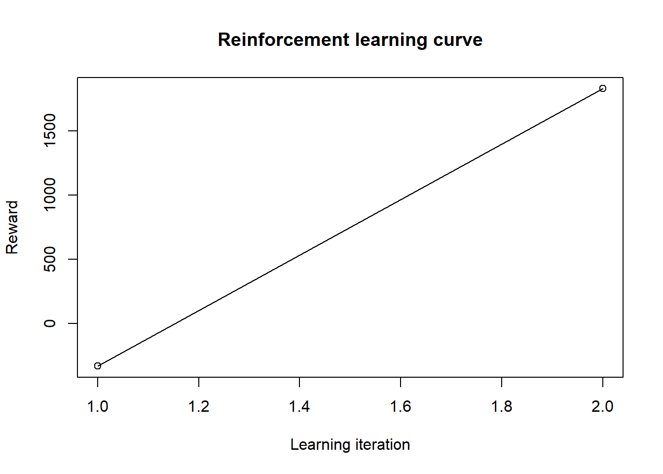
######Learn Tic-Tac-Toe
tictactoe1 = ReinforcementLearning::"tictactoe"
control1 <- list(alpha=0.2, gamma=0.4, epsilon=0.1)
set.seed(567)
model <- ReinforcementLearning(tictactoe1, s="State", a="Action", r="Reward", s_new="NextState", iter=1, control=control1)head(model$Q)## c1 c2 c3 c4 c5 c6 c7
## .XXBB..XB 0.8657823 0.00000000 0 0.00000000 0.0000000 0.0000000 0.0000000
## XXBB.B.X. 0.0000000 0.00000000 0 0.00000000 0.7378560 0.0000000 0.0000000
## .XBB..BXX -0.9980657 0.00000000 0 0.00000000 0.9940970 -0.9907766 0.0000000
## BXX...B.. 0.0000000 0.00000000 0 0.03713889 0.0000000 0.0000000 0.0000000
## ..XB..... 0.1560634 0.06396349 0 0.00000000 0.3060365 0.2643505 0.1245963
## XBXBXB... 0.0000000 0.00000000 0 0.00000000 0.0000000 0.0000000 0.9141007
## c8 c9
## .XXBB..XB 0.0000000 0.0000000
## XXBB.B.X. 0.0000000 0.0000000
## .XBB..BXX 0.0000000 0.0000000
## BXX...B.. 0.0000000 -0.2409677
## ..XB..... 0.1294771 0.1600000
## XBXBXB... 0.2199805 0.9560195plot(model$Q)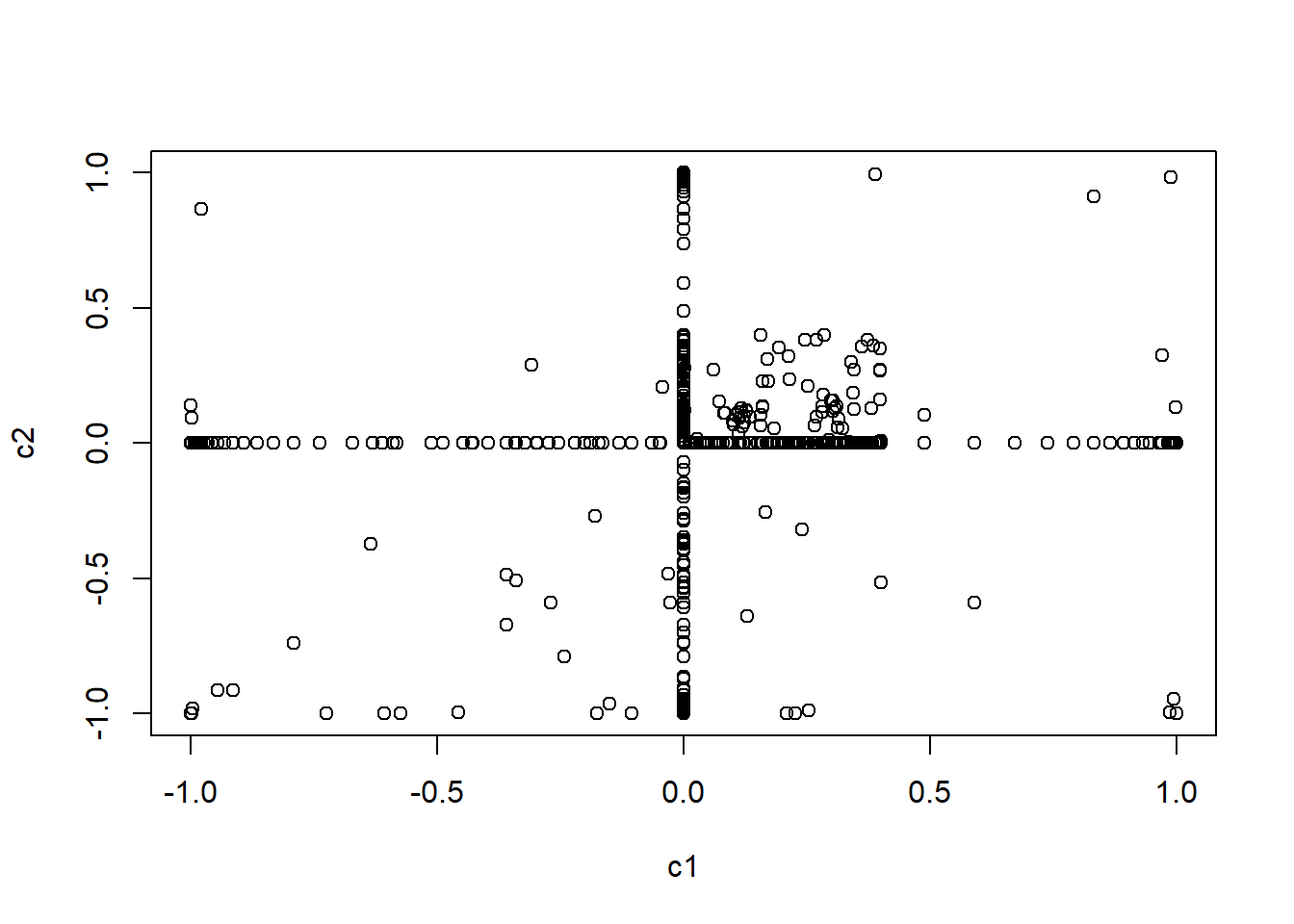
head(model$Policy)## .XXBB..XB XXBB.B.X. .XBB..BXX BXX...B.. ..XB..... XBXBXB...
## "c1" "c5" "c5" "c4" "c5" "c9"head(model$RewardSequence)## [1] 5449Here we use the Markov Decision Process or MDPtoolbox package to compare this method. At this point this is extra practice and not going to be explained due to time limitations.
###########################
library(MDPtoolbox)
#enter the probbilities of an action occuring
#Agent by column s1,s2,s3,s4
up <- matrix(c(1,0,0,0,
0.7,0.2,0.1,0,
0,0.1,0.2,0.7,
0,0,0,1), nrow=4,ncol=4,byrow=TRUE)
#when agent is in s1 and tries to go up there is a 100% prob. it will remain in s1,
#when agent is in s2 and tries to go up there is a 70% prob that it will go up to s1,
#20% prob it will remain in s2 and 10% prob it will go right to s3.
#if agent is in state s3 and tries to go up there is a 70% prob that it will go up to s4
#and a 20% prob it will remain in s3 and 10% prob it will move left to s2.
#last row if agent is in s4 and tries to go up there is a 100% prob it will remain in s4.
up## [,1] [,2] [,3] [,4]
## [1,] 1.0 0.0 0.0 0.0
## [2,] 0.7 0.2 0.1 0.0
## [3,] 0.0 0.1 0.2 0.7
## [4,] 0.0 0.0 0.0 1.0#left action probability matrix
left <- matrix(c(0.9,0.1,0,0,
0.1,0.9,0,0,
0,0.7,0.2,0.1,
0,0,0.1,0.9),
nrow=4, ncol=4, byrow=TRUE)
left## [,1] [,2] [,3] [,4]
## [1,] 0.9 0.1 0.0 0.0
## [2,] 0.1 0.9 0.0 0.0
## [3,] 0.0 0.7 0.2 0.1
## [4,] 0.0 0.0 0.1 0.9down <- matrix(c(0.3,0.7,0,0,
0,0.9,0.1,0,
0,0.1,0.9,0,
0,0,0.7,0.3),
nrow=4, ncol=4, byrow=TRUE)
down## [,1] [,2] [,3] [,4]
## [1,] 0.3 0.7 0.0 0.0
## [2,] 0.0 0.9 0.1 0.0
## [3,] 0.0 0.1 0.9 0.0
## [4,] 0.0 0.0 0.7 0.3right <- matrix(c(0.9,0.1,0,0,
0.1,0.2,0.7,0,
0,0,0.9,0.1,
0,0,0.1,0.9),
nrow=4, ncol=4,byrow=TRUE)
right## [,1] [,2] [,3] [,4]
## [1,] 0.9 0.1 0.0 0.0
## [2,] 0.1 0.2 0.7 0.0
## [3,] 0.0 0.0 0.9 0.1
## [4,] 0.0 0.0 0.1 0.9#all action matricies
up## [,1] [,2] [,3] [,4]
## [1,] 1.0 0.0 0.0 0.0
## [2,] 0.7 0.2 0.1 0.0
## [3,] 0.0 0.1 0.2 0.7
## [4,] 0.0 0.0 0.0 1.0left## [,1] [,2] [,3] [,4]
## [1,] 0.9 0.1 0.0 0.0
## [2,] 0.1 0.9 0.0 0.0
## [3,] 0.0 0.7 0.2 0.1
## [4,] 0.0 0.0 0.1 0.9down## [,1] [,2] [,3] [,4]
## [1,] 0.3 0.7 0.0 0.0
## [2,] 0.0 0.9 0.1 0.0
## [3,] 0.0 0.1 0.9 0.0
## [4,] 0.0 0.0 0.7 0.3right## [,1] [,2] [,3] [,4]
## [1,] 0.9 0.1 0.0 0.0
## [2,] 0.1 0.2 0.7 0.0
## [3,] 0.0 0.0 0.9 0.1
## [4,] 0.0 0.0 0.1 0.9#transition probabilies
T <- list(up=up, left=left, down=down, right=right)
T## $up
##      [,1] [,2] [,3] [,4]
## [1,]  1.0  0.0  0.0  0.0
## [2,]  0.7  0.2  0.1  0.0
## [3,]  0.0  0.1  0.2  0.7
## [4,]  0.0  0.0  0.0  1.0
##
## $left
##      [,1] [,2] [,3] [,4]
## [1,]  0.9  0.1  0.0  0.0
## [2,]  0.1  0.9  0.0  0.0
## [3,]  0.0  0.7  0.2  0.1
## [4,]  0.0  0.0  0.1  0.9
##
## $down
##      [,1] [,2] [,3] [,4]
## [1,]  0.3  0.7  0.0  0.0
## [2,]  0.0  0.9  0.1  0.0
## [3,]  0.0  0.1  0.9  0.0
## [4,]  0.0  0.0  0.7  0.3
##
## $right
##      [,1] [,2] [,3] [,4]
## [1,]  0.9  0.1  0.0  0.0
## [2,]  0.1  0.2  0.7  0.0
## [3,]  0.0  0.0  0.9  0.1
## [4,] 0.0 0.0 0.1 0.9#rewards matrix
R <- matrix(c(-1,-1,-1,-1,
-1,-1,-1,-1,
-1,-1,-1,-1,
10,10,10,10),
nrow=4, ncol=4,byrow=TRUE)
R## [,1] [,2] [,3] [,4]
## [1,] -1 -1 -1 -1
## [2,] -1 -1 -1 -1
## [3,] -1 -1 -1 -1
## [4,] 10 10 10 10#estimate teh policy witht the parameters and if it is a valid representation or not.
mdp_check(T, R) #empty string => ok## [1] ""#run the policy iteration and discount factor g=0.9
m <- mdp_policy_iteration(P=T, R=R, discount=0.9)
#see optimal policy and value function Vp optimal cumulative value at 100.
m## $V
## [1] 58.25663 69.09102 83.19292 100.00000
##
## $policy
## [1] 3 4 1 1
##
## $iter
## [1] 2
##
## $time
## Time difference of 0.02692699 secs#same reuslts from teh model free in Reinforcement Learning package
names(T)[m$policy]## [1] "down" "right" "up" "up"#####Bellman
P <- array(0, c(2,2,2))
P[,,1] <- matrix(c(0.5,0.5,0.8,0.2),
2,2,
byrow=TRUE)
P[,,2] <- matrix(c(0,1,0.1,0.9),
2,2,
byrow=TRUE)
P## , , 1
##
## [,1] [,2]
## [1,] 0.5 0.5
## [2,] 0.8 0.2
##
## , , 2
##
## [,1] [,2]
## [1,] 0.0 1.0
## [2,] 0.1 0.9R <- matrix(c(5,10,-1,2),
2,2,
byrow=TRUE)
R## [,1] [,2]
## [1,] 5 10
## [2,] -1 2#check valid
mdp_check(P,R)## [1] ""#The bellman function
mdp_bellman_operator(P,R, discount=0.9, Vprev= c(0,0))## $V
## [1] 10 2
##
## $policy
## [1] 2 2#with sparse matrix
P <- list()
P[[1]] <- Matrix(c(0.5,0.5,0.8,0.2),
2,2,
byrow=TRUE,
sparse=TRUE)
P[[2]] <- Matrix(c(0,1,0.1,0.9),
2,2,
byrow=TRUE,
sparse=TRUE)
P## [[1]]
## 2 x 2 sparse Matrix of class "dgCMatrix"
##
## [1,] 0.5 0.5
## [2,] 0.8 0.2
##
## [[2]]
## 2 x 2 sparse Matrix of class "dgCMatrix"
##
## [1,] . 1.0
## [2,] 0.1 0.9mdp_bellman_operator(P,R,0.9,c(0,0))## $V
## [1] 10 2
##
## $policy
## [1] 2 2##Iterative evaluation Policy
#non-sparse matrix
P <- array(0, c(2,2,2))
P[,,1] <- matrix(c(0.5,0.5,0.8,0.2),
2,2, byrow=TRUE)
P[,,2] <- matrix(c(0,1,0.1,0.9),
2,2, byrow=TRUE)
P## , , 1
##
## [,1] [,2]
## [1,] 0.5 0.5
## [2,] 0.8 0.2
##
## , , 2
##
## [,1] [,2]
## [1,] 0.0 1.0
## [2,] 0.1 0.9R <- matrix(c(5,10,-1,2),
2,2, byrow=TRUE)
R## [,1] [,2]
## [1,] 5 10
## [2,] -1 2policy <- c(2,1)
mdp_eval_policy_iterative(P,R,0.8,policy)## [1] "MDP Toolbox: iterations stopped, epsilon-optimal value function"## [,1]
## [1,] 23.17038
## [2,] 16.46307#with sparse matrix
P <- list()
P[[1]] <- Matrix(c(0.5,0.5,0.8,0.2),
2,2, byrow=TRUE, sparse=TRUE)
P[[2]] <- Matrix(c(0,1,0.1,0.9),
2,2, byrow=TRUE, sparse=TRUE)
#best value function improved
mdp_eval_policy_iterative(P,R,0.8, policy)## [1] "MDP Toolbox: iterations stopped, epsilon-optimal value function"## [,1]
## [1,] 23.17038
## [2,] 16.46307####Q-Learning
mdp_Q_learning(P,R, 0.9)## $Q
## [,1] [,2]
## [1,] 39.60663 42.91324
## [2,] 36.70754 34.68137
##
## $V
## [1] 42.91324 36.70754
##
## $policy
## [1] 2 1
##
## $mean_discrepancy
## [1] NA 0.229582566 0.158993669 0.132612875 0.109984390 0.108971178
## [7] 0.093437298 0.079662600 0.074039782 0.070305812 0.063117428 0.072237158
## [13] 0.060465963 0.055841182 0.056556994 0.050311490 0.057406442 0.051980600
## [19] 0.050117002 0.046448119 0.044027381 0.037871903 0.041540237 0.040468557
## [25] 0.038420314 0.035968831 0.029678566 0.028303595 0.029988425 0.030458720
## [31] 0.027706088 0.022090119 0.023171573 0.029378945 0.024303920 0.023737150
## [37] 0.021779496 0.022038083 0.019152821 0.021840068 0.032223175 0.019759866
## [43] 0.016278287 0.019865682 0.018222188 0.020040065 0.016805161 0.016799716
## [49] 0.015262233 0.014895981 0.020269458 0.015831233 0.014092542 0.014727892
## [55] 0.014795710 0.013610768 0.015433435 0.015925096 0.014574270 0.015518334
## [61] 0.018210295 0.014681977 0.014846452 0.012217637 0.014331745 0.014285907
## [67] 0.013305633 0.015046095 0.013428802 0.016439349 0.011110604 0.013486973
## [73] 0.015773390 0.014311491 0.013889014 0.011943958 0.012019572 0.009638250
## [79] 0.011913730 0.012324130 0.009475239 0.014902163 0.012605537 0.012467319
## [85] 0.013601543 0.013771875 0.011545978 0.012371510 0.010673475 0.011202095
## [91] 0.009906047 0.008270072 0.010256127 0.011612499 0.009108448 0.011830618
## [97] 0.009989051 0.011500018 0.009179530 0.009244230