Exploring the data with base R functions
The purpose of this post is to show the basic fucntions in R to start a data analysis project. I look at the iris dataset that comes with Rstudio shown below.
This briefly covers head(), str(), attributes(), summary(), dim(), names(), indexing [], table(), and plot() functions that come with base R. Simple to use.
Load the iris dataset
data("iris") head()
Look at the iris dataset with the head() function and lists the first five rows.
head(iris) ## Sepal.Length Sepal.Width Petal.Length Petal.Width Species
## 1 5.1 3.5 1.4 0.2 setosa
## 2 4.9 3.0 1.4 0.2 setosa
## 3 4.7 3.2 1.3 0.2 setosa
## 4 4.6 3.1 1.5 0.2 setosa
## 5 5.0 3.6 1.4 0.2 setosa
## 6 5.4 3.9 1.7 0.4 setosastr()
View the structure of the dataset. 150 objects and 5 variables.
str(iris) ## 'data.frame': 150 obs. of 5 variables:
## $ Sepal.Length: num 5.1 4.9 4.7 4.6 5 5.4 4.6 5 4.4 4.9 ...
## $ Sepal.Width : num 3.5 3 3.2 3.1 3.6 3.9 3.4 3.4 2.9 3.1 ...
## $ Petal.Length: num 1.4 1.4 1.3 1.5 1.4 1.7 1.4 1.5 1.4 1.5 ...
## $ Petal.Width : num 0.2 0.2 0.2 0.2 0.2 0.4 0.3 0.2 0.2 0.1 ...
## $ Species : Factor w/ 3 levels "setosa","versicolor",..: 1 1 1 1 1 1 1 1 1 1 ...attributes()
View the object attributes.
attributes(iris)## $names
## [1] "Sepal.Length" "Sepal.Width" "Petal.Length" "Petal.Width" "Species"
##
## $class
## [1] "data.frame"
##
## $row.names
## [1] 1 2 3 4 5 6 7 8 9 10 11 12 13 14 15 16 17 18
## [19] 19 20 21 22 23 24 25 26 27 28 29 30 31 32 33 34 35 36
## [37] 37 38 39 40 41 42 43 44 45 46 47 48 49 50 51 52 53 54
## [55] 55 56 57 58 59 60 61 62 63 64 65 66 67 68 69 70 71 72
## [73] 73 74 75 76 77 78 79 80 81 82 83 84 85 86 87 88 89 90
## [91] 91 92 93 94 95 96 97 98 99 100 101 102 103 104 105 106 107 108
## [109] 109 110 111 112 113 114 115 116 117 118 119 120 121 122 123 124 125 126
## [127] 127 128 129 130 131 132 133 134 135 136 137 138 139 140 141 142 143 144
## [145] 145 146 147 148 149 150summary()
Here is the summary statistics. Min/Max, Mean/Median, Quantiles, also a place to see if there is missing data (NA) which there is none in this iris data set.
summary(iris) ## Sepal.Length Sepal.Width Petal.Length Petal.Width
## Min. :4.300 Min. :2.000 Min. :1.000 Min. :0.100
## 1st Qu.:5.100 1st Qu.:2.800 1st Qu.:1.600 1st Qu.:0.300
## Median :5.800 Median :3.000 Median :4.350 Median :1.300
## Mean :5.843 Mean :3.057 Mean :3.758 Mean :1.199
## 3rd Qu.:6.400 3rd Qu.:3.300 3rd Qu.:5.100 3rd Qu.:1.800
## Max. :7.900 Max. :4.400 Max. :6.900 Max. :2.500
## Species
## setosa :50
## versicolor:50
## virginica :50
##
##
## dim()
names()
We can use the dim() function, names() function to view this information. Which str() did for use above more completely.
dim(iris) ## [1] 150 5names(iris)## [1] "Sepal.Length" "Sepal.Width" "Petal.Length" "Petal.Width" "Species"index [a,b]
Below is the view of rows and columns and shows the proper syntax for doing this. [12,2] is the index for row 12 column 2 of the data frame.
iris[12, 2]## [1] 3.4Or you can view row 12 in total by indexing [12, ]
iris[12, ] ## Sepal.Length Sepal.Width Petal.Length Petal.Width Species
## 12 4.8 3.4 1.6 0.2 setosaYou can index into the middle and view rows 10 through 15.
iris[10:15, ] ## Sepal.Length Sepal.Width Petal.Length Petal.Width Species
## 10 4.9 3.1 1.5 0.1 setosa
## 11 5.4 3.7 1.5 0.2 setosa
## 12 4.8 3.4 1.6 0.2 setosa
## 13 4.8 3.0 1.4 0.1 setosa
## 14 4.3 3.0 1.1 0.1 setosa
## 15 5.8 4.0 1.2 0.2 setosaHere is the way to view column 5.
iris[ ,5]## [1] setosa setosa setosa setosa setosa setosa
## [7] setosa setosa setosa setosa setosa setosa
## [13] setosa setosa setosa setosa setosa setosa
## [19] setosa setosa setosa setosa setosa setosa
## [25] setosa setosa setosa setosa setosa setosa
## [31] setosa setosa setosa setosa setosa setosa
## [37] setosa setosa setosa setosa setosa setosa
## [43] setosa setosa setosa setosa setosa setosa
## [49] setosa setosa versicolor versicolor versicolor versicolor
## [55] versicolor versicolor versicolor versicolor versicolor versicolor
## [61] versicolor versicolor versicolor versicolor versicolor versicolor
## [67] versicolor versicolor versicolor versicolor versicolor versicolor
## [73] versicolor versicolor versicolor versicolor versicolor versicolor
## [79] versicolor versicolor versicolor versicolor versicolor versicolor
## [85] versicolor versicolor versicolor versicolor versicolor versicolor
## [91] versicolor versicolor versicolor versicolor versicolor versicolor
## [97] versicolor versicolor versicolor versicolor virginica virginica
## [103] virginica virginica virginica virginica virginica virginica
## [109] virginica virginica virginica virginica virginica virginica
## [115] virginica virginica virginica virginica virginica virginica
## [121] virginica virginica virginica virginica virginica virginica
## [127] virginica virginica virginica virginica virginica virginica
## [133] virginica virginica virginica virginica virginica virginica
## [139] virginica virginica virginica virginica virginica virginica
## [145] virginica virginica virginica virginica virginica virginica
## Levels: setosa versicolor virginicaView rows 1, 5, 19, 15 and the respective column variables.
iris[c(1,5,10,15), ] ## Sepal.Length Sepal.Width Petal.Length Petal.Width Species
## 1 5.1 3.5 1.4 0.2 setosa
## 5 5.0 3.6 1.4 0.2 setosa
## 10 4.9 3.1 1.5 0.1 setosa
## 15 5.8 4.0 1.2 0.2 setosaOr view rows 1, 5, 10, 15 in column 1 only. Note by default this converts the column to a row in R.
iris[c(1,5,10,15), 1]## [1] 5.1 5.0 4.9 5.8table()
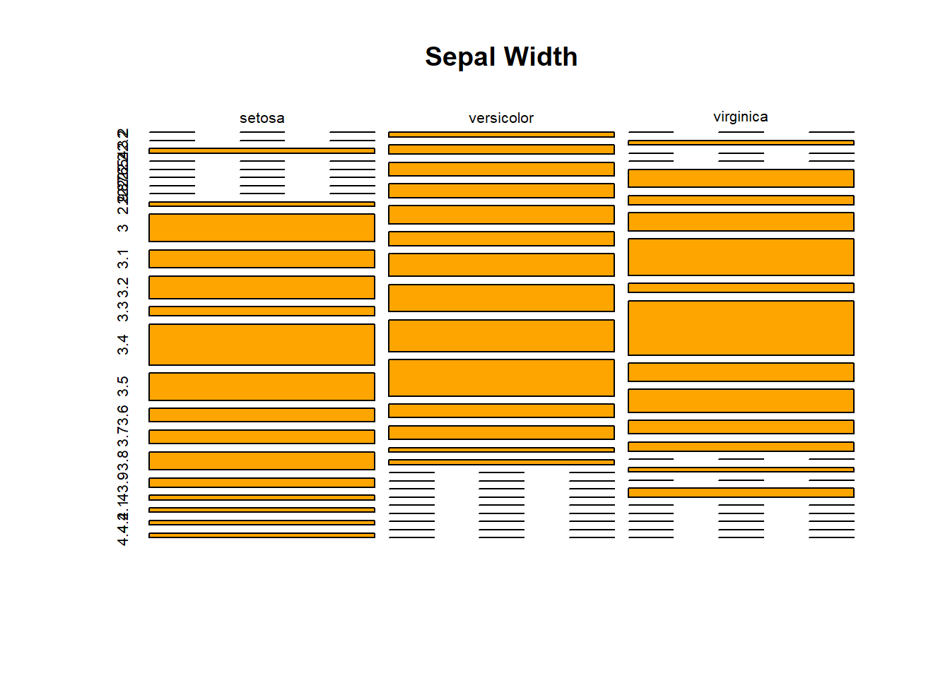
Here we can view the data in a table and basic plot. The tables show the three categorical variables (factors in R) and Petal.Width and Sepal.Width variables (integers). We can see a pattern develop with each Species/Petal.Width and Species/Sepal.Width when plotted.
table(iris$Species, iris$Petal.Width)##
## 0.1 0.2 0.3 0.4 0.5 0.6 1 1.1 1.2 1.3 1.4 1.5 1.6 1.7 1.8 1.9 2
## setosa 5 29 7 7 1 1 0 0 0 0 0 0 0 0 0 0 0
## versicolor 0 0 0 0 0 0 7 3 5 13 7 10 3 1 1 0 0
## virginica 0 0 0 0 0 0 0 0 0 0 1 2 1 1 11 5 6
##
## 2.1 2.2 2.3 2.4 2.5
## setosa 0 0 0 0 0
## versicolor 0 0 0 0 0
## virginica 6 3 8 3 3petwidth <- table(iris$Species, iris$Petal.Width)plot()
The plot is multi-dimensional.
barplot(petwidth, main = "Petal Width")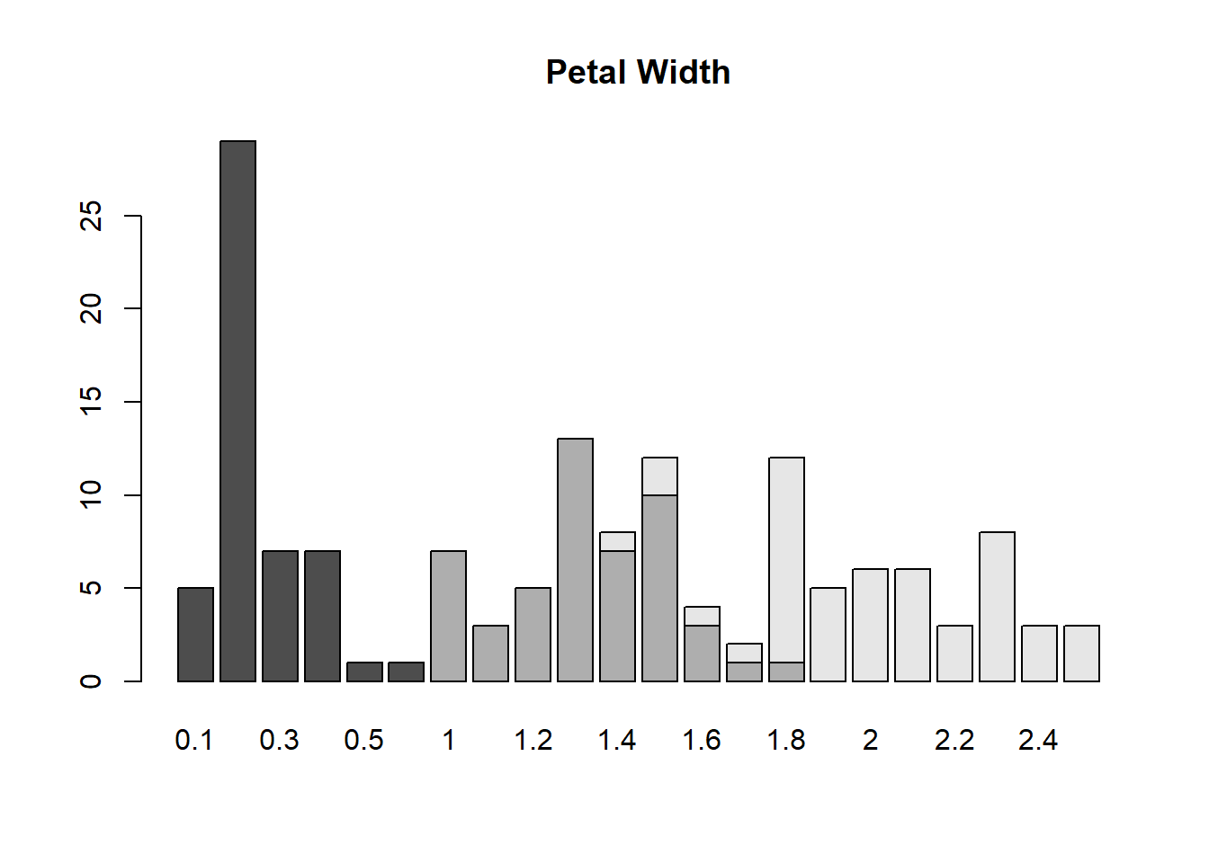
plot(petwidth, main = "Petal Width", col = "green")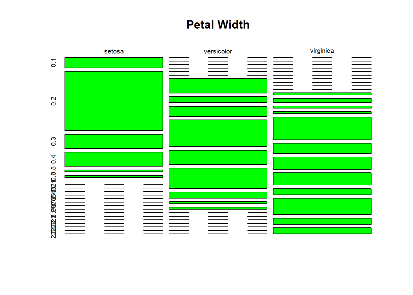
table()
table(iris$Species, iris$Sepal.Width)##
## 2 2.2 2.3 2.4 2.5 2.6 2.7 2.8 2.9 3 3.1 3.2 3.3 3.4 3.5 3.6 3.7
## setosa 0 0 1 0 0 0 0 0 1 6 4 5 2 9 6 3 3
## versicolor 1 2 3 3 4 3 5 6 7 8 3 3 1 1 0 0 0
## virginica 0 1 0 0 4 2 4 8 2 12 4 5 3 2 0 1 0
##
## 3.8 3.9 4 4.1 4.2 4.4
## setosa 4 2 1 1 1 1
## versicolor 0 0 0 0 0 0
## virginica 2 0 0 0 0 0sepwidth <- table(iris$Species, iris$Sepal.Width)plot()
barplot(sepwidth, main = "Sepal Width")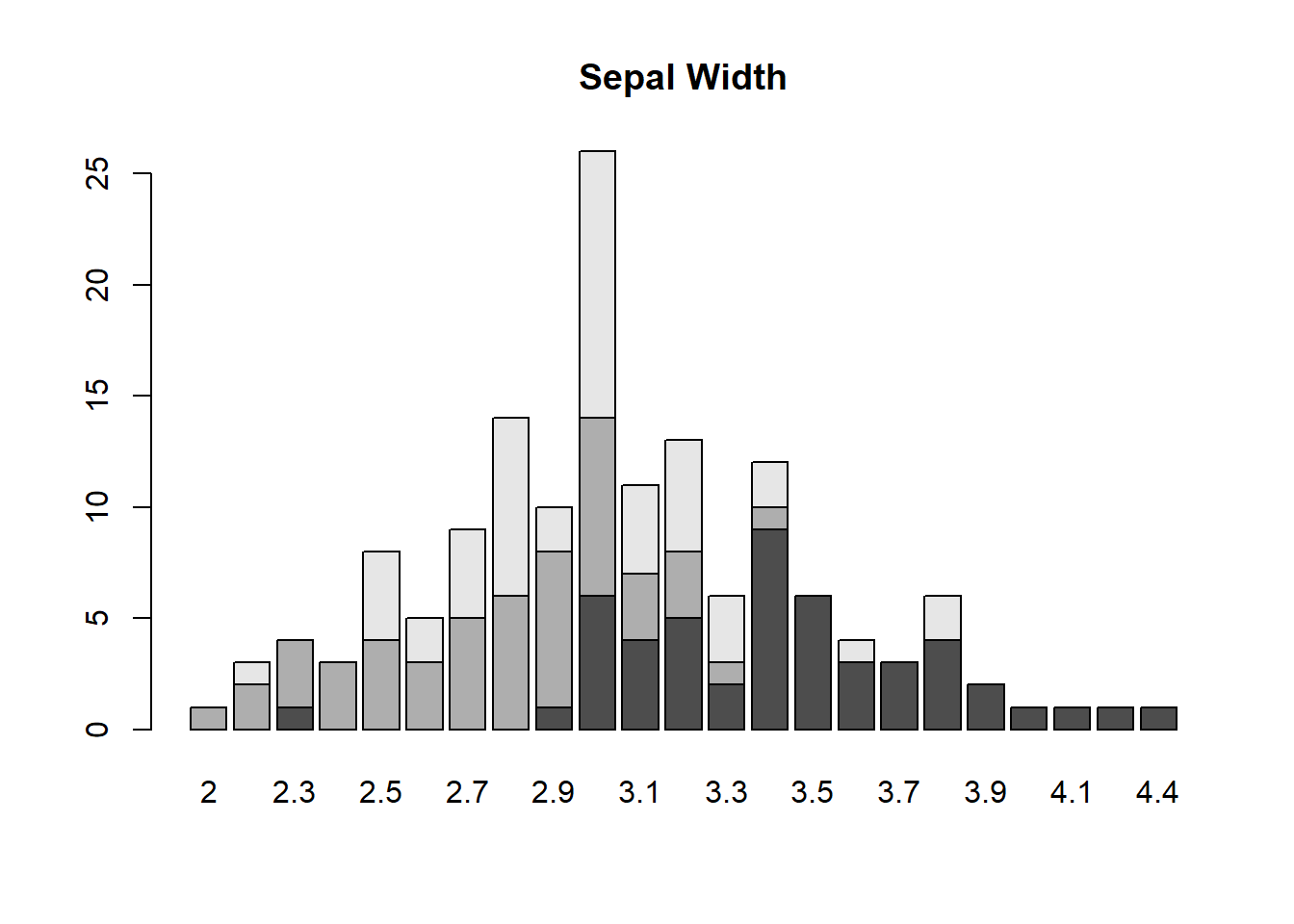
plot(sepwidth, main = "Sepal Width", col = "orange")