K-Means Clustering
The first section uses the iris data set and k-means clustering starting with 3 cluster centers and an nstart of 15. The results are displayed below in the fit object. There are 3 clusters sized 50, 62, and 38. The within sum of squares by cluster is 88.4% and the smaller number (15.15, 39.82, & 23.87) indicates how closely related objects are in the clusters. The first cluster has the most related objects and the second cluster has the lesser of related objects mostly taken from the third cluster.
library(tidyverse)
library(factoextra)
library(cluster)
library(fpc)
library(GGally)
library(data.table)
set.seed(22)
str(iris)#view data## 'data.frame': 150 obs. of 5 variables:
## $ Sepal.Length: num 5.1 4.9 4.7 4.6 5 5.4 4.6 5 4.4 4.9 ...
## $ Sepal.Width : num 3.5 3 3.2 3.1 3.6 3.9 3.4 3.4 2.9 3.1 ...
## $ Petal.Length: num 1.4 1.4 1.3 1.5 1.4 1.7 1.4 1.5 1.4 1.5 ...
## $ Petal.Width : num 0.2 0.2 0.2 0.2 0.2 0.4 0.3 0.2 0.2 0.1 ...
## $ Species : Factor w/ 3 levels "setosa","versicolor",..: 1 1 1 1 1 1 1 1 1 1 ...iris1 <- select(iris, -Species)#remove non-numeric factor variable
fit <- kmeans(iris1, 3, nstart=15)#start with 3 centers and 15 random sets chosen
fit #view data## K-means clustering with 3 clusters of sizes 38, 50, 62
##
## Cluster means:
## Sepal.Length Sepal.Width Petal.Length Petal.Width
## 1 6.850000 3.073684 5.742105 2.071053
## 2 5.006000 3.428000 1.462000 0.246000
## 3 5.901613 2.748387 4.393548 1.433871
##
## Clustering vector:
## [1] 2 2 2 2 2 2 2 2 2 2 2 2 2 2 2 2 2 2 2 2 2 2 2 2 2 2 2 2 2 2 2 2 2 2 2 2 2
## [38] 2 2 2 2 2 2 2 2 2 2 2 2 2 3 3 1 3 3 3 3 3 3 3 3 3 3 3 3 3 3 3 3 3 3 3 3 3
## [75] 3 3 3 1 3 3 3 3 3 3 3 3 3 3 3 3 3 3 3 3 3 3 3 3 3 3 1 3 1 1 1 1 3 1 1 1 1
## [112] 1 1 3 3 1 1 1 1 3 1 3 1 3 1 1 3 3 1 1 1 1 1 3 1 1 1 1 3 1 1 1 3 1 1 1 3 1
## [149] 1 3
##
## Within cluster sum of squares by cluster:
## [1] 23.87947 15.15100 39.82097
## (between_SS / total_SS = 88.4 %)
##
## Available components:
##
## [1] "cluster" "centers" "totss" "withinss" "tot.withinss"
## [6] "betweenss" "size" "iter" "ifault"fit$withinss #view within sum of squares## [1] 23.87947 15.15100 39.82097fit$betweenss #view between cluster sum of squares## [1] 602.5192barplot(t(fit$centers), beside=TRUE, xlab="Cluster", ylab="Value") #inspect the center of each cluster with barplot method.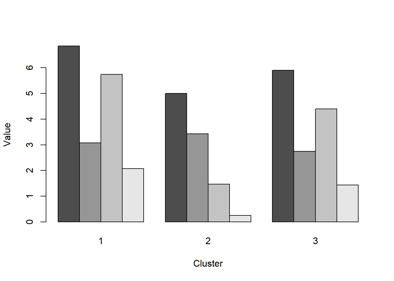
plot(iris1, fit$centers)# plot out centers matrix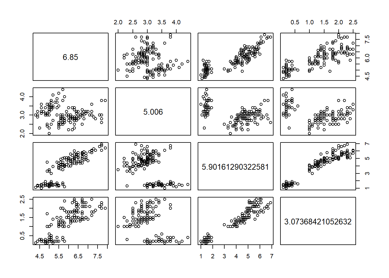
plot(iris1, col=fit$cluster, pch=19, cex=0.75)# same plot but colored for clarity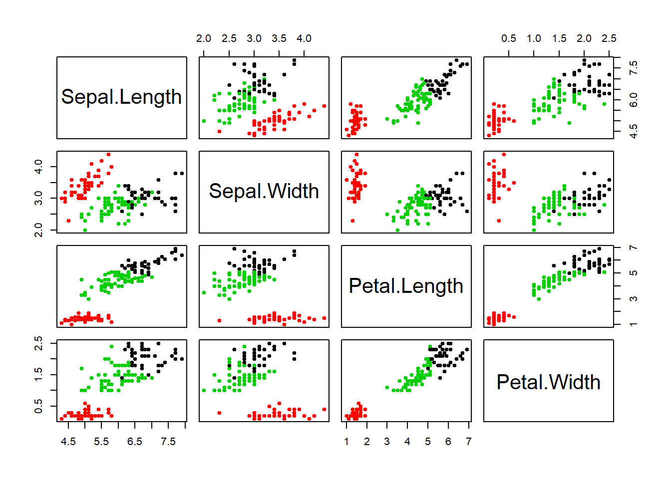
Here I scale the iris data and run the kmeans again with 3 centers and 15 random set. The plot shows each cluster circle, square, triangle -color coded, and the center of the cluster with a larger symbol. The ellipse helps to define the boundaries of the cluster.
iris.scaled <- scale(iris1)#scale numeric data
km.res <- eclust(iris.scaled, "kmeans", k=3, nstart=15, graph=FALSE)#run k-means again on scaled data
fviz_cluster(km.res, geom="point", ellipse.type="norm", main="k-means cluster")# a very nice plot from this package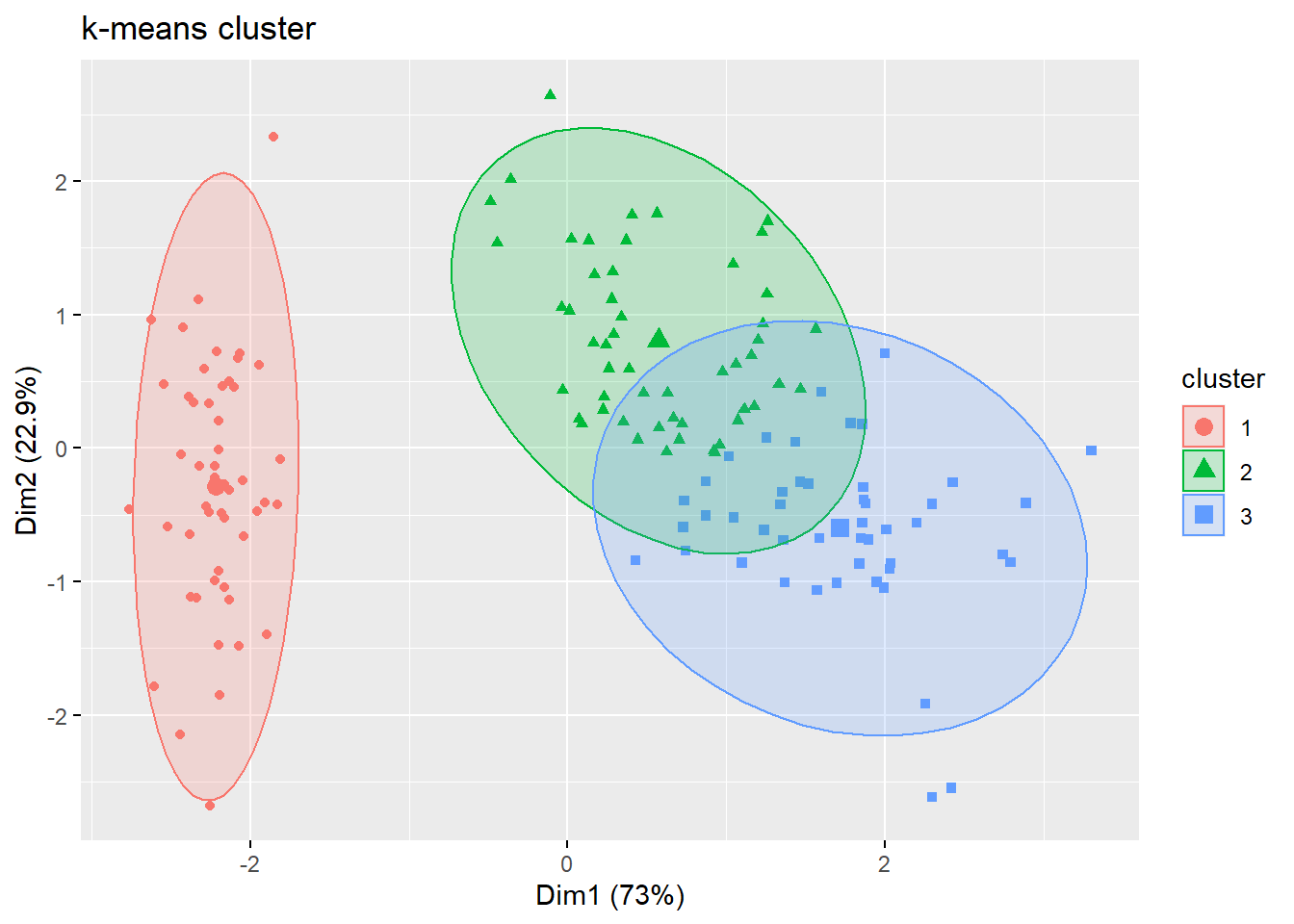
clusplot(iris.scaled, fit$cluster, color=TRUE, shade=TRUE)#another package and way to view the same data cluster, no centers shown 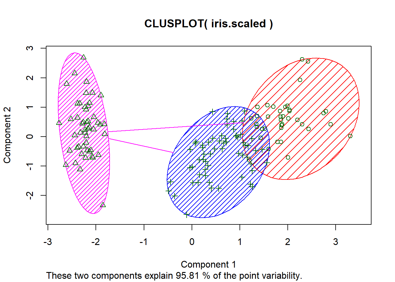
mds <- cmdscale(dist(iris.scaled), k=3)#more of the same but different method. plot(mds, col=fit$cluster, pch=19, cex=0.75)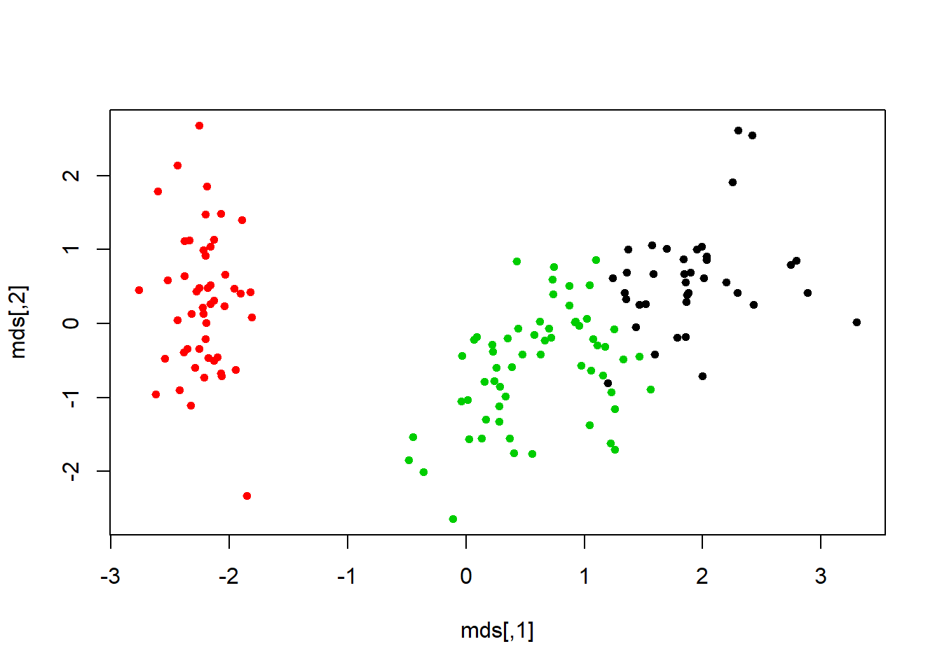
The silhouette shows how closely related the point are in the cluster. The value closer to 1 is the better cluster and cluster 1 is at 0.79 (best) and cluster two id 0.21 (worst).
cs <- cluster.stats(dist(iris.scaled), fit$cluster)#cluster fitting
fits <- silhouette(fit$cluster, dist(iris1))#how well do the clusters fit
summary(fits)#quick summary to show silhouette values.## Silhouette of 150 units in 3 clusters from silhouette.default(x = fit$cluster, dist = dist(iris1)) :
## Cluster sizes and average silhouette widths:
## 38 50 62
## 0.4511051 0.7981405 0.4173199
## Individual silhouette widths:
## Min. 1st Qu. Median Mean 3rd Qu. Max.
## 0.02636 0.39115 0.56231 0.55282 0.77552 0.85391plot(fits) #graph the silhouette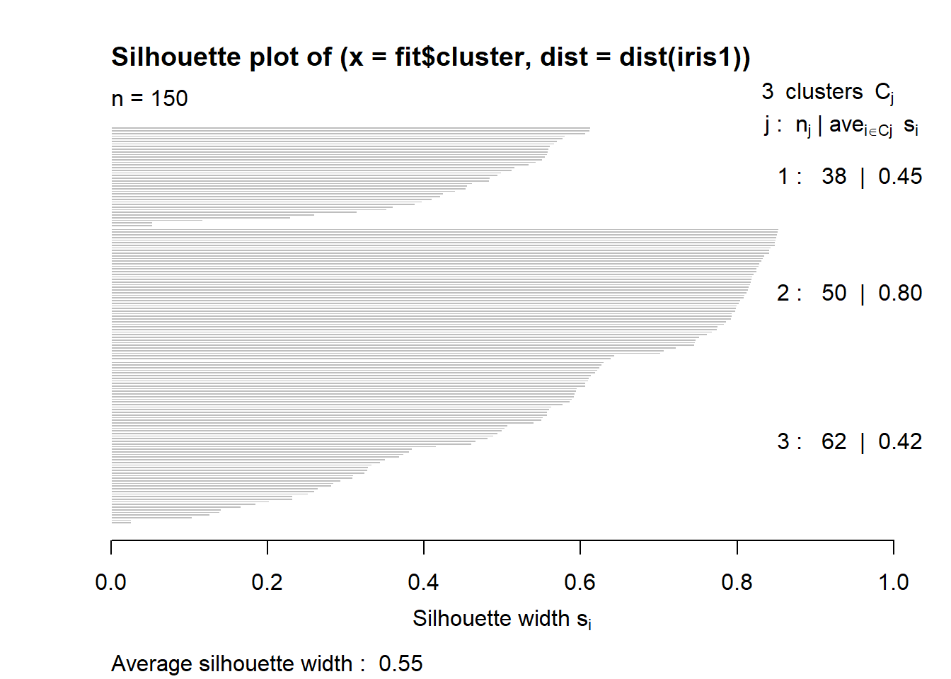
This graph shows the optimal number of clusters. A sharp decline after 2 clusters indicates 2 may be the better choice for number of clusters.
nk <- 2:15 #show 2 to 15 clusters
set.seed(22)
WSS <- sapply(nk, function(k) {kmeans(iris1, centers=k)$tot.withinss})
WSS
## [1] 152.34795 78.85144 57.26562 50.13655 47.65657 37.59074 36.26302
## [8] 28.81355 26.08442 24.98467 25.05792 25.65793 21.66389 20.76329plot(nk, WSS, type="l", xlab="Number of k", ylab="within sum of squares", lwd=2, col="red")# graphing the optimal number of clusters. 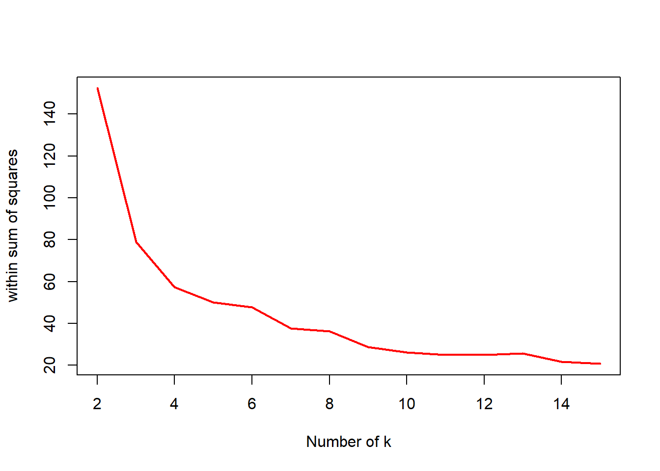
SW <- sapply(nk, function(k) {
  cluster.stats(dist(iris1), kmeans(iris1, centers=k)$cluster)$avg.silwidth})
SW
## [1] 0.6810462 0.5528190 0.4104276 0.3727767 0.3664804 0.3588294 0.3266471
## [8] 0.3227828 0.3177546 0.3049373 0.3193459 0.2968904 0.2492297 0.2618958plot(nk, SW, type="l", xlab="Number of Clusters", ylab="average silhoutte width", lwd=2, col="firebrick3")#confirm above 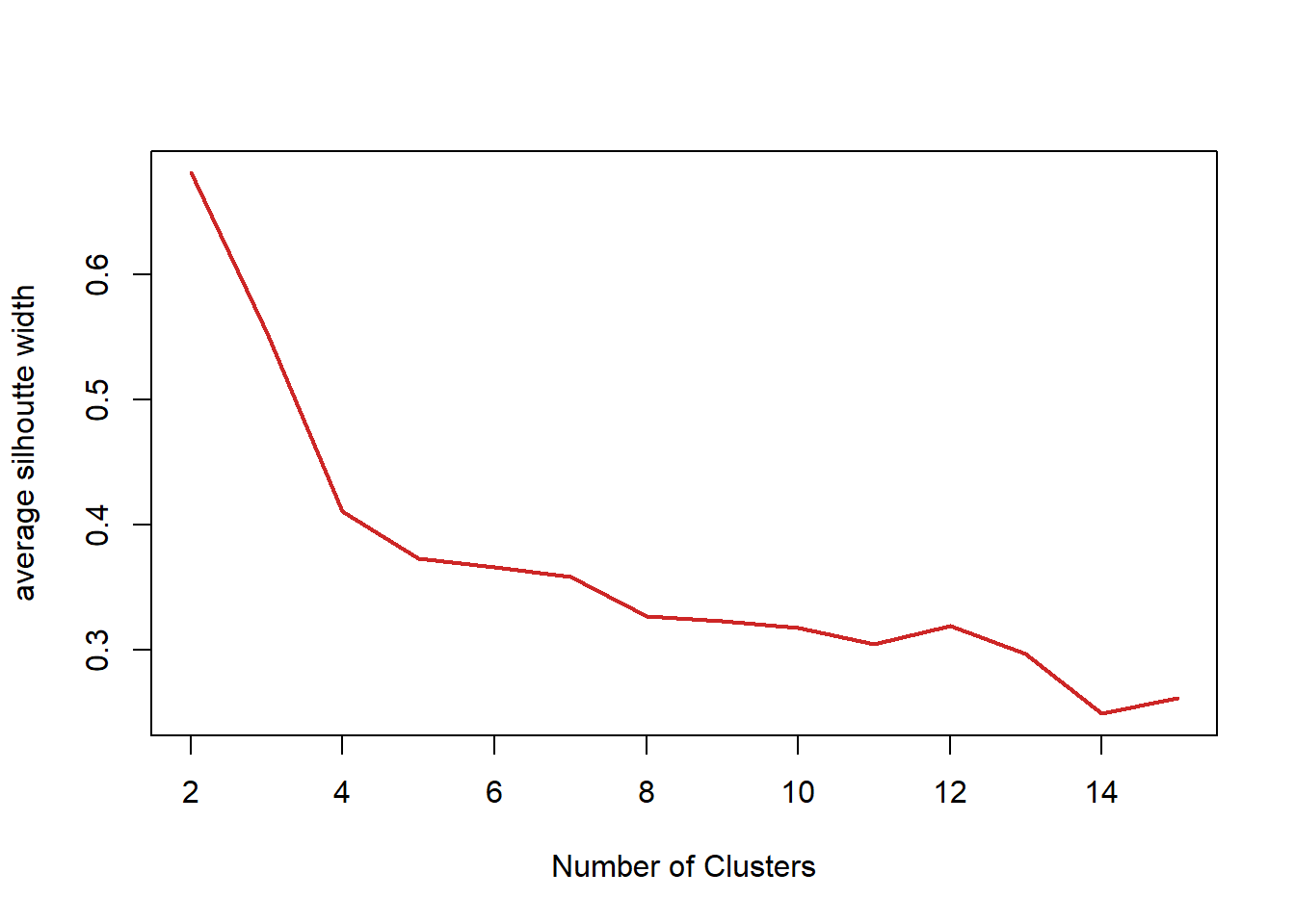
To confirm the graph above, the max amount of clusters shall be 2 for the best results.
nk[which.max(SW)]# what is the optimal number of clusters?## [1] 2fit2 <- kmeans(iris1, 2)#2 clusters is optimal
fit2#show data of 2 clusters. cluster 1 at 28 is best## K-means clustering with 2 clusters of sizes 97, 53
##
## Cluster means:
## Sepal.Length Sepal.Width Petal.Length Petal.Width
## 1 6.301031 2.886598 4.958763 1.695876
## 2 5.005660 3.369811 1.560377 0.290566
##
## Clustering vector:
## [1] 2 2 2 2 2 2 2 2 2 2 2 2 2 2 2 2 2 2 2 2 2 2 2 2 2 2 2 2 2 2 2 2 2 2 2 2 2
## [38] 2 2 2 2 2 2 2 2 2 2 2 2 2 1 1 1 1 1 1 1 2 1 1 1 1 1 1 1 1 1 1 1 1 1 1 1 1
## [75] 1 1 1 1 1 1 1 1 1 1 1 1 1 1 1 1 1 1 1 2 1 1 1 1 2 1 1 1 1 1 1 1 1 1 1 1 1
## [112] 1 1 1 1 1 1 1 1 1 1 1 1 1 1 1 1 1 1 1 1 1 1 1 1 1 1 1 1 1 1 1 1 1 1 1 1 1
## [149] 1 1
##
## Within cluster sum of squares by cluster:
## [1] 123.79588 28.55208
## (between_SS / total_SS = 77.6 %)
##
## Available components:
##
## [1] "cluster" "centers" "totss" "withinss" "tot.withinss"
## [6] "betweenss" "size" "iter" "ifault"plot(iris1, col=fit2$cluster, pch=19, cex=0.75)# plotting the 2 clusters in color. 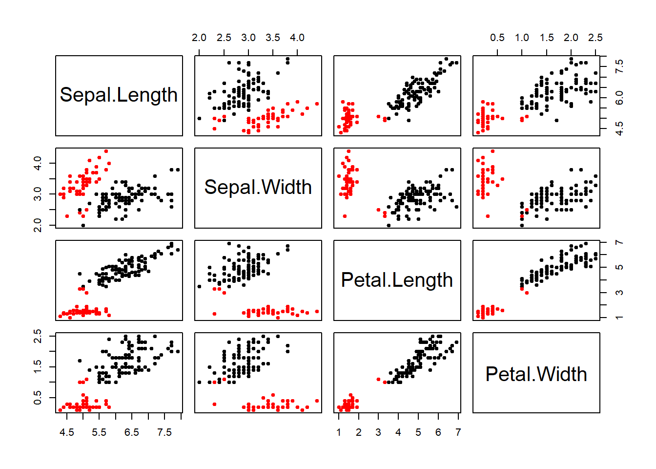
Biopsy Data - KMeans Clustering
This section looks at the biopsy data set and we look for the optimal number of clusters like we did above on the iris data set.
biopsy <- read.csv("http://wilkelab.org/classes/SDS348/data_sets/biopsy.csv")#read in biopsy datastr(biopsy)#view data## 'data.frame': 683 obs. of 10 variables:
## $ clump_thickness : int 5 5 3 6 4 8 1 2 2 4 ...
## $ uniform_cell_size : int 1 4 1 8 1 10 1 1 1 2 ...
## $ uniform_cell_shape : int 1 4 1 8 1 10 1 2 1 1 ...
## $ marg_adhesion : int 1 5 1 1 3 8 1 1 1 1 ...
## $ epithelial_cell_size: int 2 7 2 3 2 7 2 2 2 2 ...
## $ bare_nuclei : int 1 10 2 4 1 10 10 1 1 1 ...
## $ bland_chromatin : int 3 3 3 3 3 9 3 3 1 2 ...
## $ normal_nucleoli : int 1 2 1 7 1 7 1 1 1 1 ...
## $ mitoses : int 1 1 1 1 1 1 1 1 5 1 ...
## $ outcome : Factor w/ 2 levels "benign","malignant": 1 1 1 1 1 2 1 1 1 1 ...biopsy1 <- select(biopsy, -outcome) # clear up take out factor variable
biopsy1 <- scale(biopsy1)#scale data to fitset.seed(89)
fit2 <- kmeans(biopsy1, 3, nstart=15)#start with a guess 3 centers 15 random
fit2# view kmeans biopsy results. ## K-means clustering with 3 clusters of sizes 205, 34, 444
##
## Cluster means:
## clump_thickness uniform_cell_size uniform_cell_shape marg_adhesion
## 1 0.9361869 1.0520888 1.0509572 0.8749764
## 2 1.1570335 1.7451687 1.7584806 1.5686056
## 3 -0.5208501 -0.6194007 -0.6198977 -0.5241053
## epithelial_cell_size bare_nuclei bland_chromatin normal_nucleoli mitoses
## 1 0.8557137 1.1370229 0.9991392 0.9167723 0.03192493
## 2 1.8526866 1.1500556 1.3791236 1.5649814 3.75975251
## 3 -0.5369654 -0.6130441 -0.5669228 -0.5431255 -0.30264909
##
## Clustering vector:
## [1] 3 1 3 1 3 1 3 3 3 3 3 3 3 3 1 1 3 3 1 3 1 1 3 3 3 3 3 3 3 3 3 1 3 3 3 1 3
## [38] 1 1 1 1 1 1 3 1 3 3 1 1 3 1 2 1 1 1 1 1 3 1 3 1 1 3 2 3 1 2 3 3 2 3 1 1 3
## [75] 3 3 3 3 3 3 3 3 2 2 1 1 3 3 3 3 3 3 3 3 3 3 2 1 1 3 3 1 2 3 1 1 3 1 3 1 1
## [112] 1 3 3 3 2 3 3 3 3 1 1 1 3 1 3 1 3 3 3 1 3 3 3 3 3 3 3 3 1 3 3 1 3 3 2 3 1
## [149] 1 3 3 1 3 3 2 1 3 3 3 3 1 2 3 3 3 3 3 2 1 1 3 1 3 1 3 3 3 1 1 3 1 2 1 3 1
## [186] 1 3 3 3 3 1 3 3 3 1 1 3 3 3 2 1 3 3 3 2 1 3 2 1 1 3 3 1 3 3 1 3 1 1 3 1 1
## [223] 3 1 1 1 1 1 3 2 1 2 1 3 3 3 3 3 3 1 1 3 3 1 1 1 1 1 3 3 3 1 1 2 1 1 1 3 1
## [260] 1 2 3 1 3 1 3 3 3 3 3 2 3 3 1 1 1 1 2 3 1 1 3 3 1 1 1 3 1 1 3 2 3 1 1 3 3
## [297] 1 3 3 3 1 3 3 1 1 3 1 1 3 1 3 3 1 3 1 1 1 3 3 1 1 3 1 3 3 1 1 3 3 3 1 3 3
## [334] 3 1 1 3 3 1 1 3 3 3 2 1 1 2 1 3 3 3 3 2 1 3 3 3 3 3 3 3 3 3 3 3 3 3 1 3 3
## [371] 3 3 1 3 3 3 3 1 3 3 3 3 3 3 3 3 2 3 3 3 3 3 3 3 3 3 3 1 3 1 3 1 3 3 3 3 1
## [408] 3 3 3 1 3 1 3 3 3 3 3 3 1 1 1 3 3 3 1 3 3 3 3 3 3 3 3 1 3 3 3 1 3 3 1 1 3
## [445] 3 3 3 3 3 3 1 1 1 3 3 3 3 3 3 3 3 3 3 3 1 3 3 2 1 3 3 3 2 1 3 3 1 3 1 3 3
## [482] 3 3 3 3 3 3 3 3 3 3 2 3 3 3 3 3 3 3 1 1 3 3 3 1 3 3 1 1 3 3 3 3 3 3 1 3 3
## [519] 3 3 3 3 3 3 3 3 3 3 3 3 3 1 3 3 1 3 3 3 3 3 3 3 3 3 3 3 3 3 3 3 1 3 3 1 1
## [556] 1 1 3 3 1 3 3 3 3 3 3 1 1 3 3 3 1 3 1 3 1 1 1 3 1 3 3 3 3 3 3 3 3 1 1 1 3
## [593] 3 1 3 1 1 2 3 3 3 3 3 3 3 3 3 3 3 3 1 3 3 3 3 3 3 1 3 3 1 3 3 3 3 3 3 3 3
## [630] 3 3 3 2 3 3 3 3 3 3 3 3 1 1 3 3 3 3 3 3 3 3 3 1 1 1 3 3 3 3 3 3 3 3 3 2 1
## [667] 3 3 3 3 3 3 3 3 3 1 3 3 3 3 1 1 1
##
## Within cluster sum of squares by cluster:
## [1] 1485.9547 266.8739 482.2359
## (between_SS / total_SS = 63.6 %)
##
## Available components:
##
## [1] "cluster" "centers" "totss" "withinss" "tot.withinss"
## [6] "betweenss" "size" "iter" "ifault"barplot(t(fit2$centers), beside=TRUE, xlab="Cluster", ylab="Value")#barplot the centers.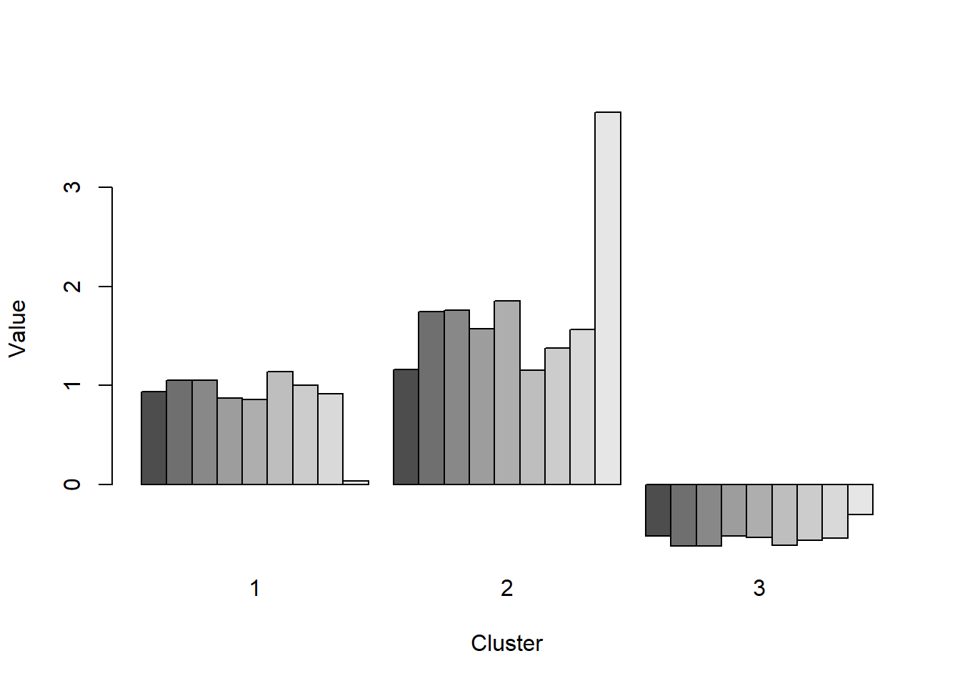
plot(biopsy1, col=fit2$cluster, pch=17, cex=1)#scatter plot the clusters. 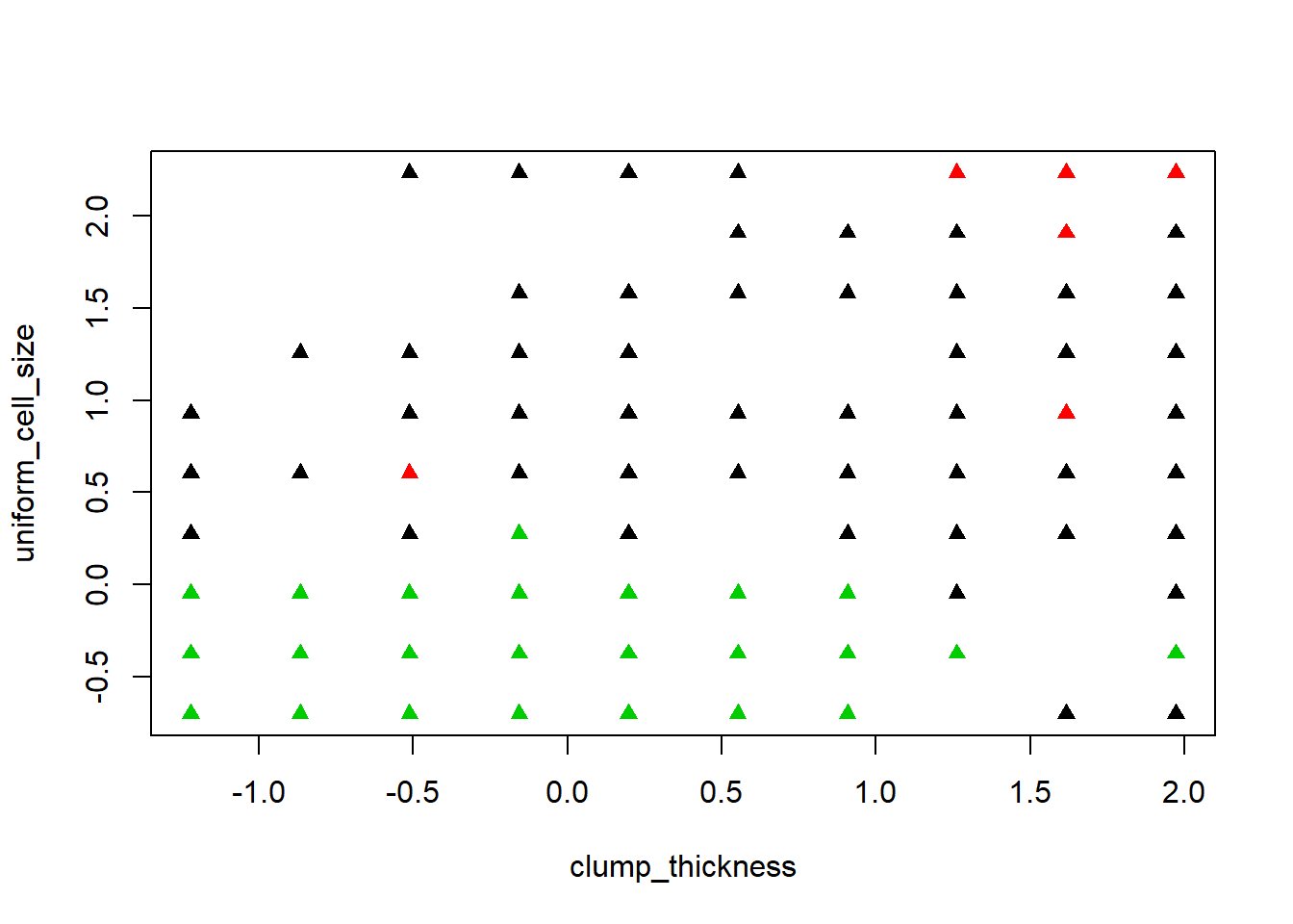
clusplot(biopsy1, fit2$cluster, color=TRUE, col.p="black",shade=TRUE, labels=4 ,main = "Cluster Plot for Biopsy Data")#cluster plot from earlier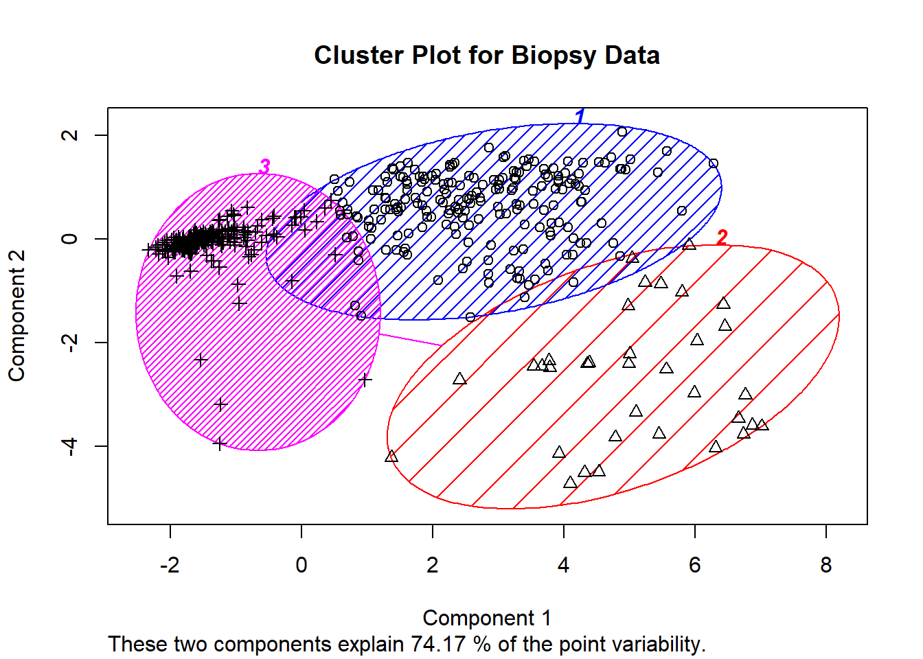
mds <- cmdscale(dist(biopsy1), k=3)plot(mds, col=fit2$cluster, pch=17, cex=0.75)#another way to view cluster plot. 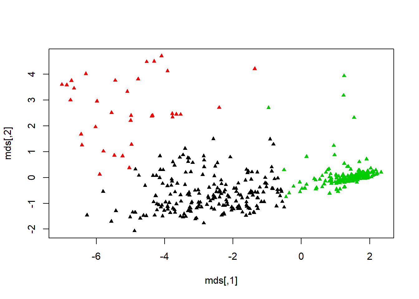
cs <- cluster.stats
fits2 <- silhouette(fit2$cluster, dist(biopsy1))
summary(fits2)#important summary showing silhouette values. ## Silhouette of 683 units in 3 clusters from silhouette.default(x = fit2$cluster, dist = dist(biopsy1)) :
## Cluster sizes and average silhouette widths:
## 205 34 444
## 0.1933782 0.2837312 0.7470335
## Individual silhouette widths:
## Min. 1st Qu. Median Mean 3rd Qu. Max.
## -0.2024 0.2853 0.7332 0.5578 0.7930 0.8289Here we look at the optimal number of clusters for the biopsy data set. The graph is similar to the iris data set with a shape decline after 2 clusters. We can confirm that 2 cluster is the optimal for the biopsy data below.
nk <- 2:15
set.seed(22)
WSS <- sapply(nk, function(k) {kmeans(biopsy1, centers=k)$tot.withinss})
WSS
## [1] 2724.155 2573.039 1942.554 1827.404 1722.914 1630.802 1659.516 1541.870
## [9] 1433.658 1408.762 1382.666 1337.406 1326.605 1251.217plot(nk, WSS, type="l", xlab="Number of k", ylab="within sum of squares", lwd=2, col="slateblue3")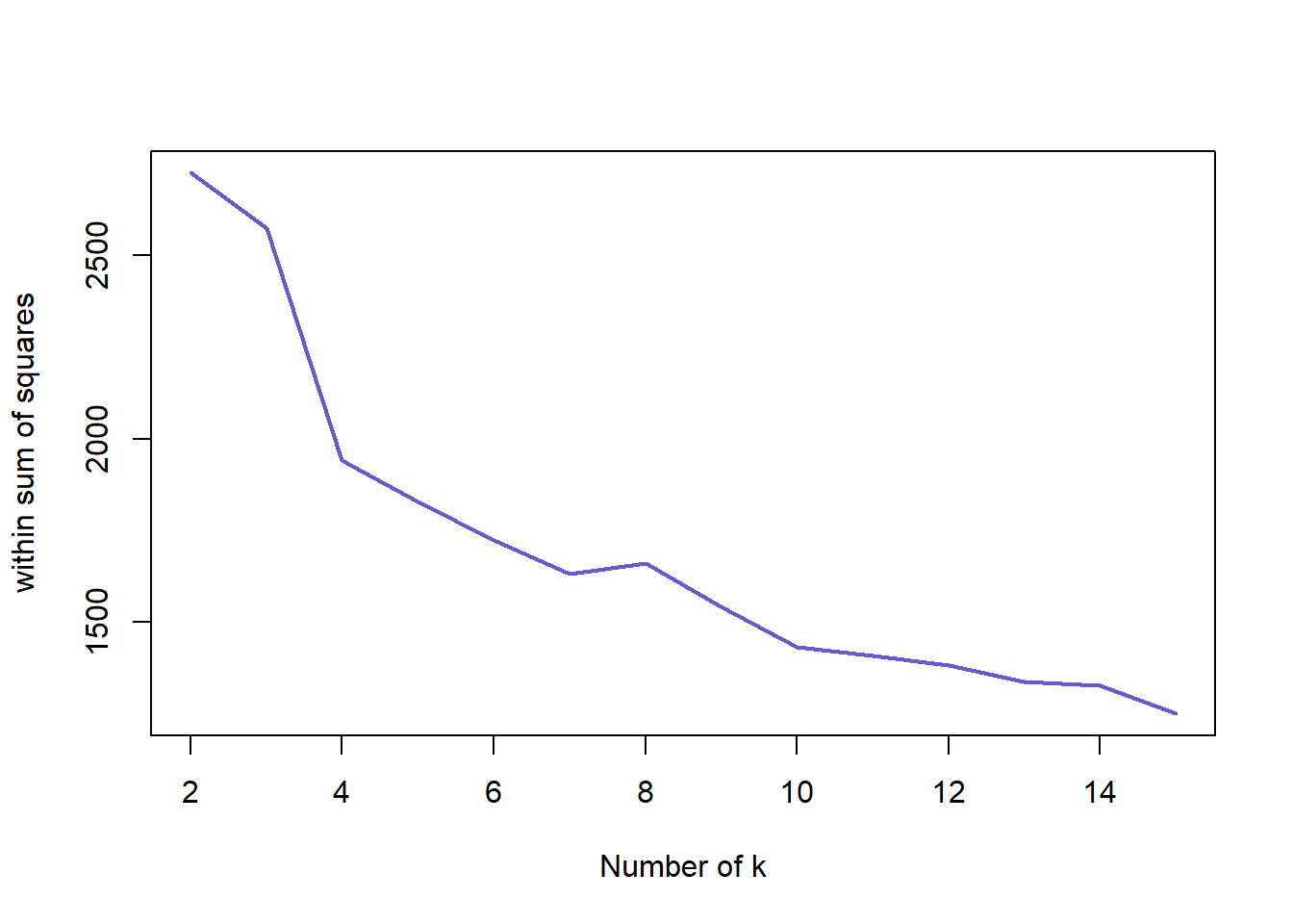
SW <- sapply(nk, function(k) {
  cluster.stats(dist(biopsy1), kmeans(biopsy1, centers=k)$cluster)$avg.silwidth})
SW
## [1] 0.5732451 0.2623748 0.2357959 0.2442259 0.4878855 0.1829936 0.1854109
## [8] 0.2009834 0.1804915 0.1687851 0.1866895 0.2029021 0.2329044 0.1769594plot(nk, SW, type="l", xlab="Number of CLusters", ylab="average silhoutte width", lwd=2, col="springgreen3")#plot out 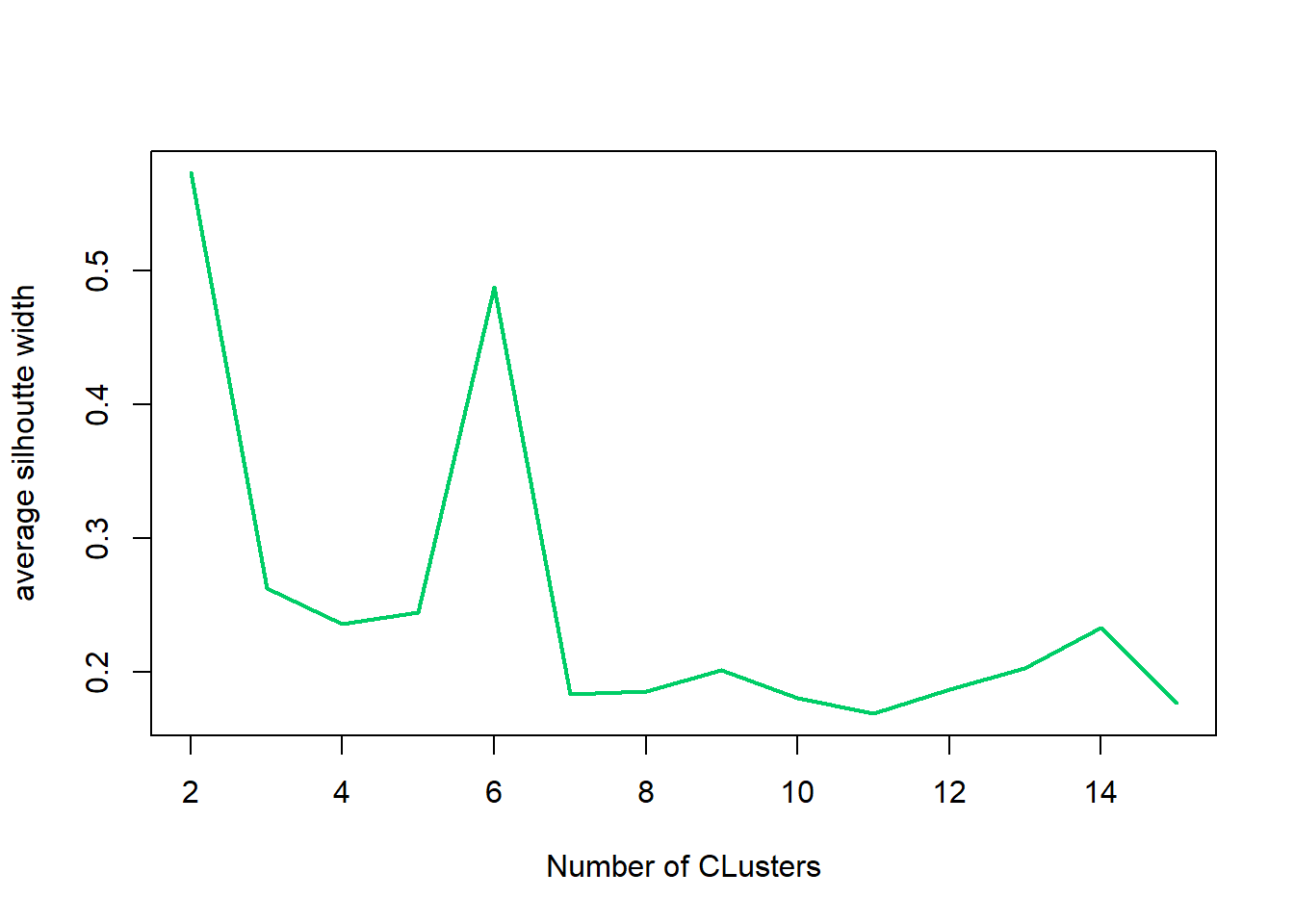
Optimal number of clusters is 2 with k-means and the biopsy data set.
nk[which.max(SW)]## [1] 2This section show all the work performed doing the exercises for week 6. Most is a repeat of what is done above with a slightly different way of looking at the data graphically.
theme_set(theme_bw(base_size=12))

iris %>% select(-Species) %>%
  kmeans(centers=3) ->
  km
km
## K-means clustering with 3 clusters of sizes 38, 62, 50
##
## Cluster means:
##   Sepal.Length Sepal.Width Petal.Length Petal.Width
## 1     6.850000    3.073684     5.742105    2.071053
## 2     5.901613    2.748387     4.393548    1.433871
## 3     5.006000    3.428000     1.462000    0.246000
##
## Clustering vector:
##   [1] 3 3 3 3 3 3 3 3 3 3 3 3 3 3 3 3 3 3 3 3 3 3 3 3 3 3 3 3 3 3 3 3 3 3 3 3 3
##  [38] 3 3 3 3 3 3 3 3 3 3 3 3 3 2 2 1 2 2 2 2 2 2 2 2 2 2 2 2 2 2 2 2 2 2 2 2 2
##  [75] 2 2 2 1 2 2 2 2 2 2 2 2 2 2 2 2 2 2 2 2 2 2 2 2 2 2 1 2 1 1 1 1 2 1 1 1 1
## [112] 1 1 2 2 1 1 1 1 2 1 2 1 2 1 1 2 2 1 1 1 1 1 2 1 1 1 1 2 1 1 1 2 1 1 1 2 1
## [149] 1 2
##
## Within cluster sum of squares by cluster:
## [1] 23.87947 39.82097 15.15100
## (between_SS / total_SS = 88.4 %)
##
## Available components:
##
## [1] "cluster" "centers" "totss" "withinss" "tot.withinss"
## [6] "betweenss" "size" "iter" "ifault"km$centers## Sepal.Length Sepal.Width Petal.Length Petal.Width
## 1 6.850000 3.073684 5.742105 2.071053
## 2 5.901613 2.748387 4.393548 1.433871
## 3 5.006000 3.428000 1.462000 0.246000km$cluster## [1] 3 3 3 3 3 3 3 3 3 3 3 3 3 3 3 3 3 3 3 3 3 3 3 3 3 3 3 3 3 3 3 3 3 3 3 3 3
## [38] 3 3 3 3 3 3 3 3 3 3 3 3 3 2 2 1 2 2 2 2 2 2 2 2 2 2 2 2 2 2 2 2 2 2 2 2 2
## [75] 2 2 2 1 2 2 2 2 2 2 2 2 2 2 2 2 2 2 2 2 2 2 2 2 2 2 1 2 1 1 1 1 2 1 1 1 1
## [112] 1 1 2 2 1 1 1 1 2 1 2 1 2 1 1 2 2 1 1 1 1 1 2 1 1 1 1 2 1 1 1 2 1 1 1 2 1
## [149] 1 2iris_clustered <- data.frame(iris, cluster=factor(km$cluster))ggplot(iris_clustered,
aes(x=Petal.Width,
y=Sepal.Width,
color=cluster,
shape=Species)) +
geom_point()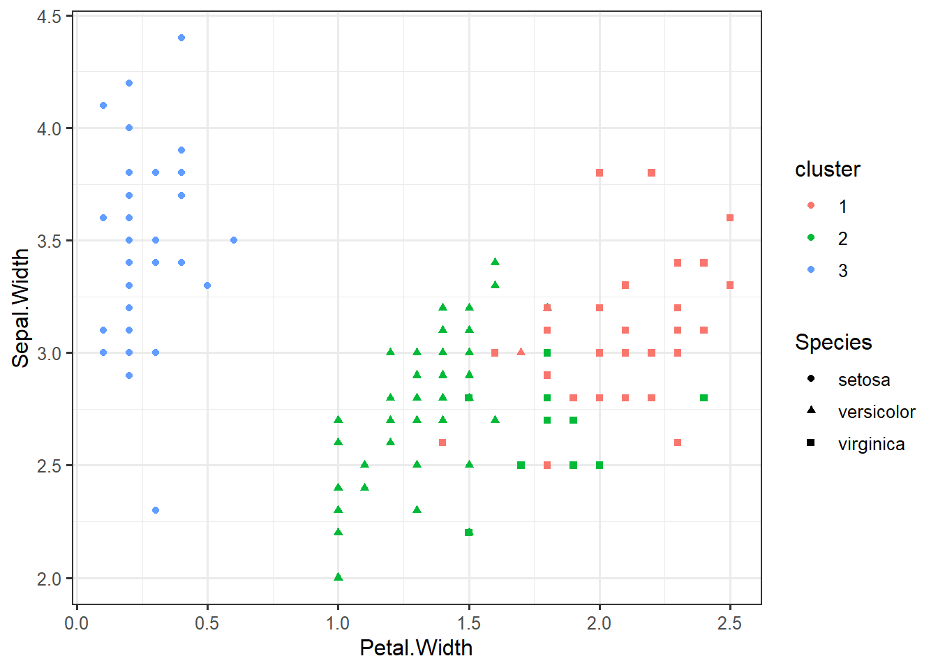
iris %>% select(-Species) %>% kmeans(centers=3) -> km
iris_clustered <- data.frame(iris, cluster=factor(km$cluster))
ggplot(iris_clustered,
aes(x=Petal.Width,
y=Sepal.Width,
color=cluster,
shape=Species)) +
geom_point()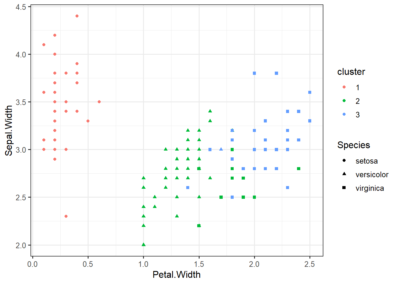
iris %>% select(-Species) %>% kmeans(centers=3, nstart=10) -> km
iris_clustered <- data.frame(iris, cluster=factor(km$cluster))
ggplot(iris_clustered,
aes(x=Petal.Width,
y=Sepal.Width,
color=cluster,
shape=Species)) +
geom_point()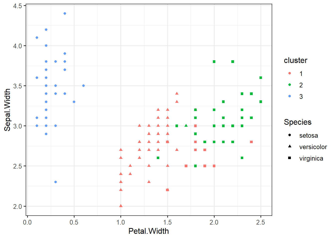
iris_numeric <- select(iris, -Species)
wss <- (nrow(iris_numeric)-1)*sum(apply(iris_numeric, 2, var))
        for (i in 2:15) wss[i] <- sum(kmeans(iris_numeric,
                                             nstart=10,
                                             centers=i)$withinss)
wss_data <- data.frame(centers=1:15, wss)
ggplot(wss_data,
aes(x=centers, y=wss)) +
geom_point() +
geom_line() +
xlab("Number of Clusters") +
ylab("Within groups sum of squares")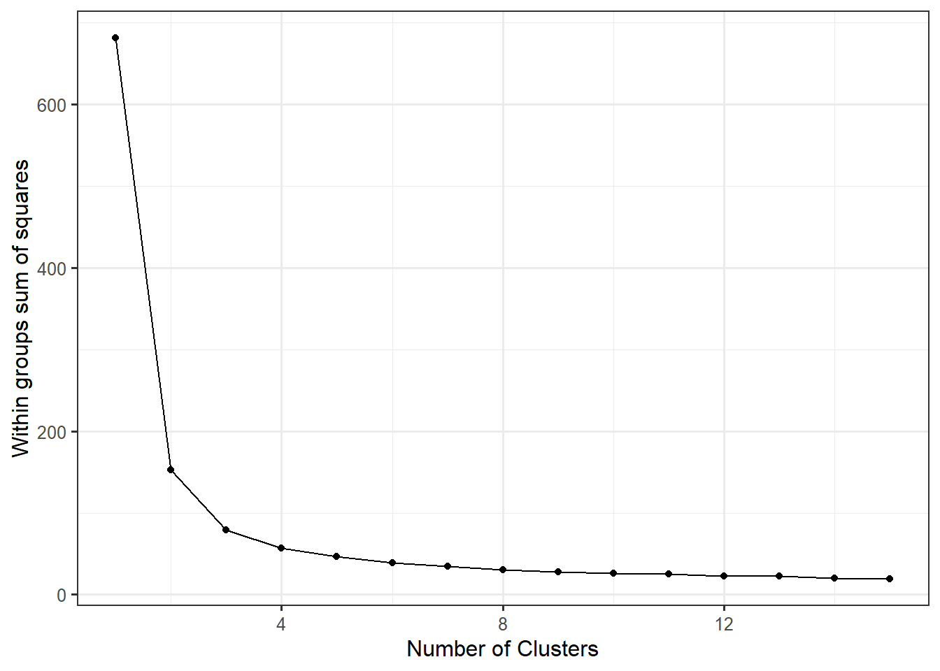
Biopsy Data Clustering
head(biopsy) ## clump_thickness uniform_cell_size uniform_cell_shape marg_adhesion
## 1 5 1 1 1
## 2 5 4 4 5
## 3 3 1 1 1
## 4 6 8 8 1
## 5 4 1 1 3
## 6 8 10 10 8
## epithelial_cell_size bare_nuclei bland_chromatin normal_nucleoli mitoses
## 1 2 1 3 1 1
## 2 7 10 3 2 1
## 3 2 2 3 1 1
## 4 3 4 3 7 1
## 5 2 1 3 1 1
## 6 7 10 9 7 1
## outcome
## 1 benign
## 2 benign
## 3 benign
## 4 benign
## 5 benign
## 6 malignantbiopsy %>%
select(-outcome) %>%
scale() %>%
prcomp() -> pca
biopsy %>%
select(-outcome) %>%
kmeans(centers=2, nstart=10) -> km
cluster_data <- data.frame(pca$x, cluster=factor(km$cluster), outcome=biopsy$outcome)ggplot(cluster_data,
aes(x=PC1, y=PC2,
color=cluster,
shape=outcome)) +
geom_point()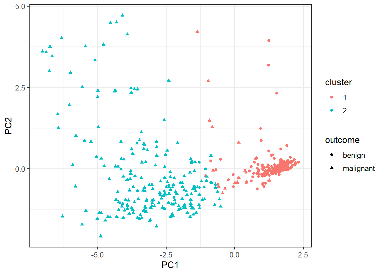
biopsy %>%
  select(-outcome) %>%
  kmeans(centers=3, nstart=10) -> km

cluster_data <- data.frame(pca$x, cluster=factor(km$cluster), outcome=biopsy$outcome)
ggplot(cluster_data,
aes(x=PC1, y=PC2,
color=cluster,
shape=outcome)) +
geom_point()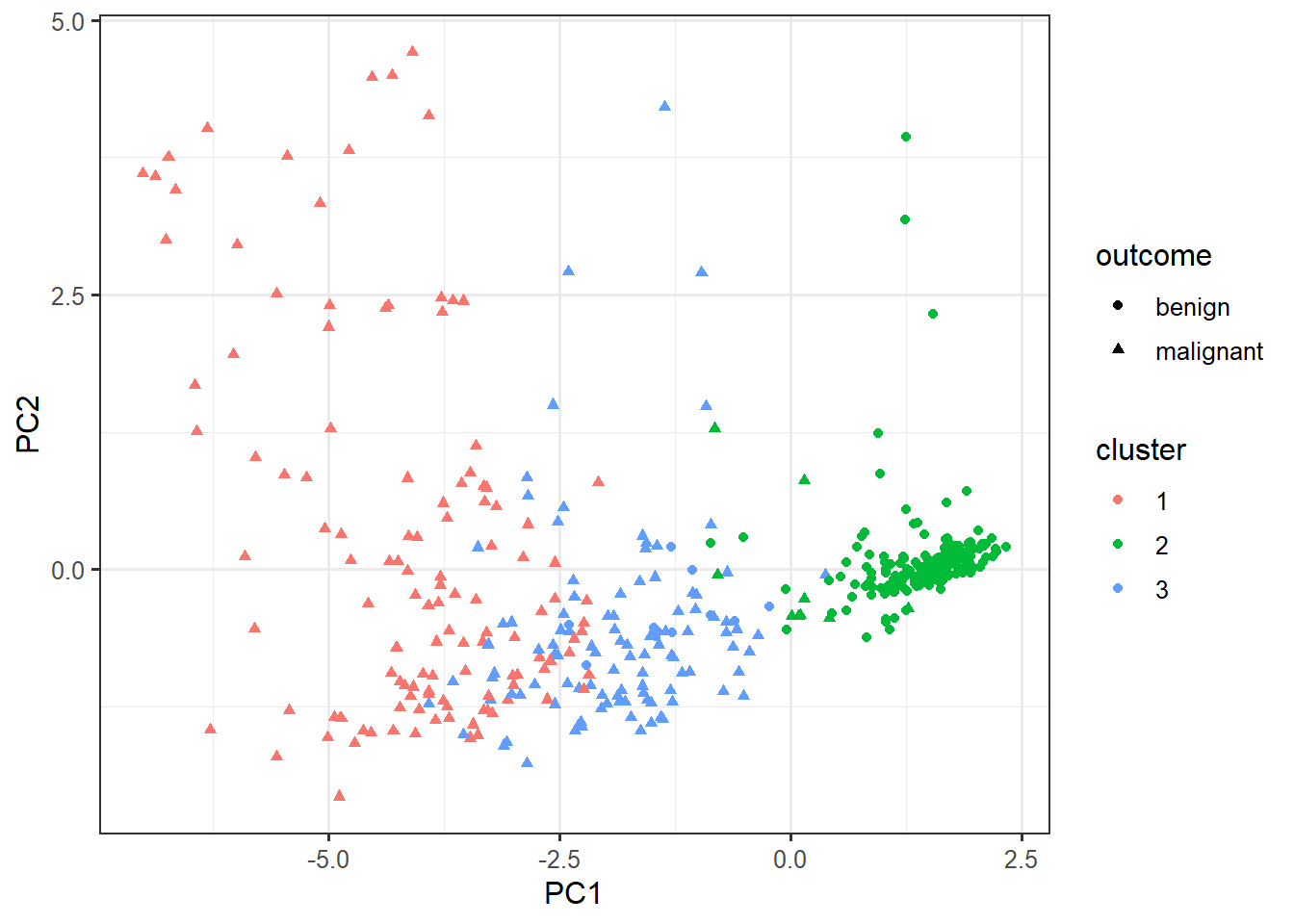
biopsy %>%
  select(-outcome) %>%
  kmeans(centers=4, nstart=10) -> km

cluster_data <- data.frame(pca$x, cluster=factor(km$cluster), outcome=biopsy$outcome)
ggplot(cluster_data,
aes(x=PC1, y=PC2,
color=cluster,
shape=outcome)) +
geom_point()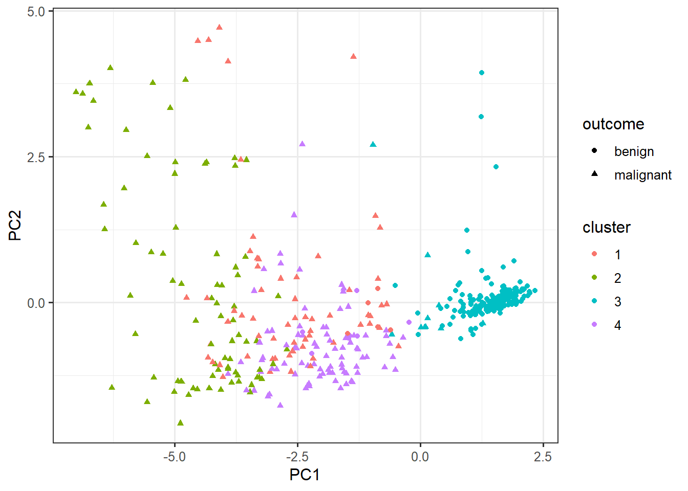
biopsy_numeric <- select(biopsy, -outcome)
wss <- (nrow(biopsy_numeric)-1)*sum(apply(biopsy_numeric, 2, var))
  for (i in 2:15) wss[i] <- sum(kmeans(biopsy_numeric,
                                       nstart=10,
                                       centers=i)$withinss)
wss_data <- data.frame(centers=1:15, wss)
ggplot(wss_data,
aes(x=centers, y=wss)) +
geom_point() +
geom_line() +
xlab("Number of Clusters") +
ylab("Within groupssum of squares") 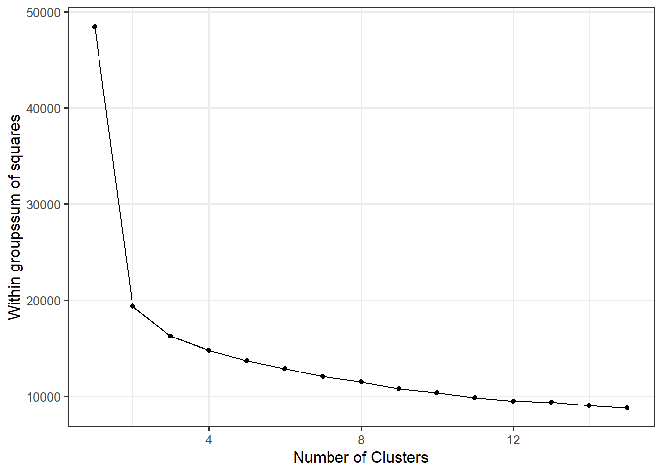
iris %>%
  select(-Species) %>%
  kmeans(centers=3, nstart=10) -> km

iris_clustered <- data.frame(iris, cluster=factor(km$cluster))
Iris Data Clustering
ggplot(iris_clustered, aes(x=Petal.Width, y=Sepal.Width, color=cluster, shape=Species)) +geom_point()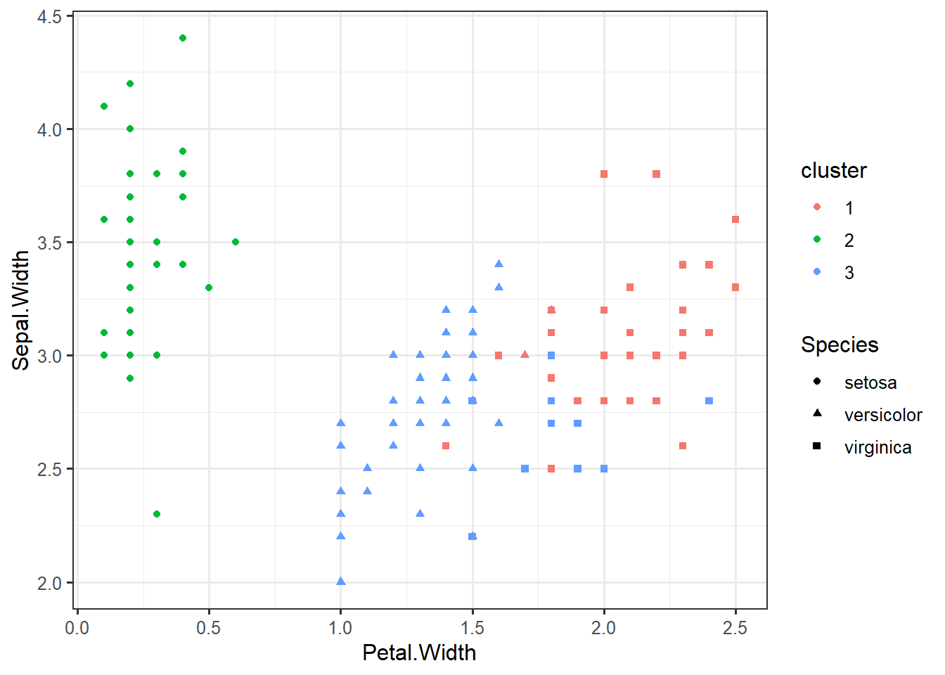
centroids <- data.frame(km$centers)
centroids
## Sepal.Length Sepal.Width Petal.Length Petal.Width
## 1 6.850000 3.073684 5.742105 2.071053
## 2 5.006000 3.428000 1.462000 0.246000
## 3 5.901613 2.748387 4.393548 1.433871centroids <- data.frame(centroids, cluster=factor(1:3))ggplot(iris_clustered,
aes(x=Petal.Width,
y=Sepal.Width,
color=cluster)) +
geom_point(aes(shape=Species)) +
geom_point(data=centroids,
aes(fill=cluster),
shape=21,
color="black",
size=4,
stroke=1)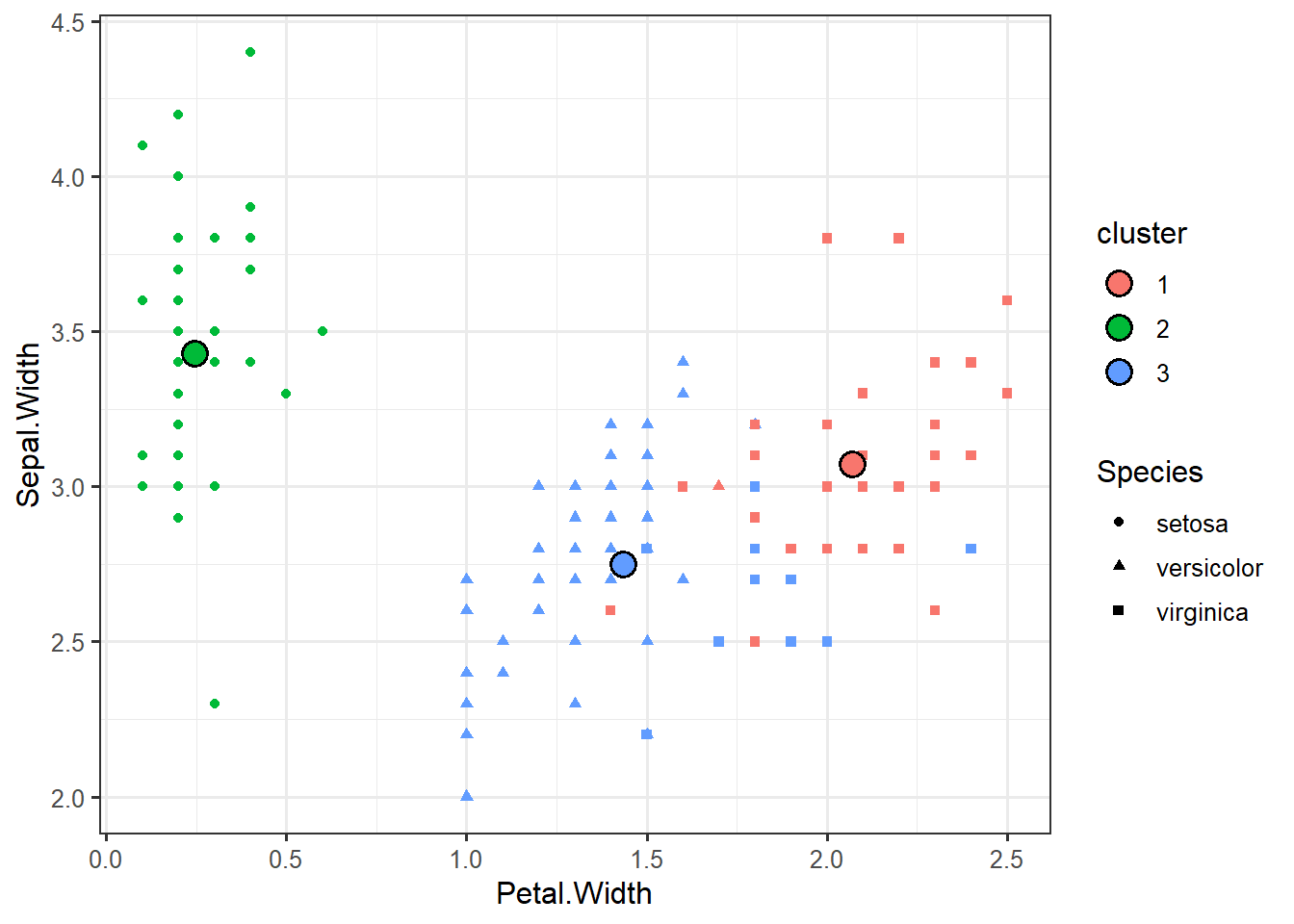
data_iris <- data.table(iris)ggpairs(data_iris, columns=1:5, mapping=aes(colour=Species))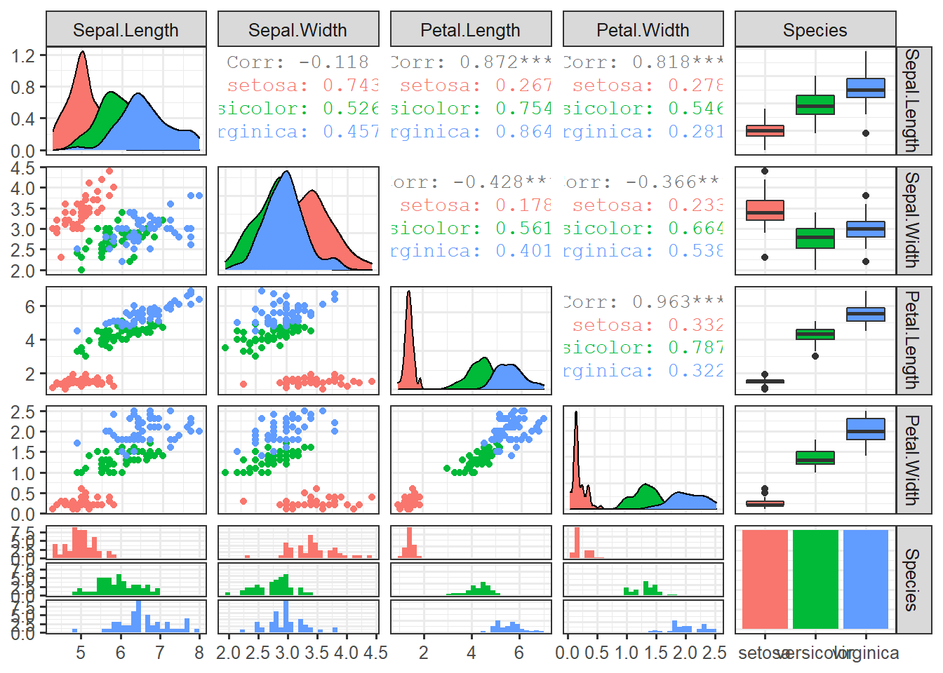
set.seed(123)
not_norm_clusters <- kmeans(data_iris[,1:4, with=F], 3)
data_iris$cluster <- as.factor(not_norm_clusters$cluster)
ggpairs(data_iris, columns=1:5, mapping=aes(colour=cluster))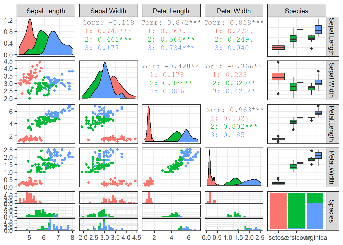
norm_cluster <- kmeans(scale(data_iris[,1:4, with=F], scale=T), 3)
data_iris$cluster <- as.factor(norm_cluster$cluster)
ggpairs(data_iris, clolumns=1:5, mapping=aes(colour=cluster))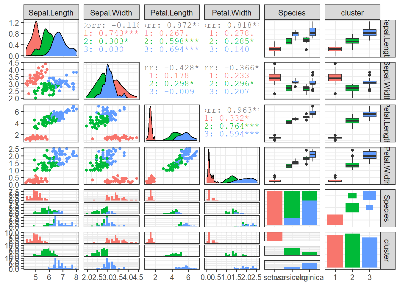
set.seed(456)
performance <- c()
for (i in rep(1:100, times=30)) {
  clust <- kmeans(data_iris[,1:4, with=F],i)
  performance <- c(performance, 1-clust$tot.withinss/clust$totss)
}

perf_df <- data.frame(metrics=performance, number_of_center=rep(1:100, times=30))
ggplot(perf_df,
aes(x=number_of_center, y=metrics)) +
geom_point(alpha=0.2) +
geom_vline(xintercept=3,
color='red')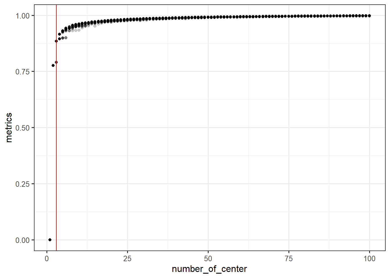
head(iris)## Sepal.Length Sepal.Width Petal.Length Petal.Width Species
## 1 5.1 3.5 1.4 0.2 setosa
## 2 4.9 3.0 1.4 0.2 setosa
## 3 4.7 3.2 1.3 0.2 setosa
## 4 4.6 3.1 1.5 0.2 setosa
## 5 5.0 3.6 1.4 0.2 setosa
## 6 5.4 3.9 1.7 0.4 setosaggplot(iris,
aes(Petal.Length,
Petal.Width,
color=Species)) +
geom_point()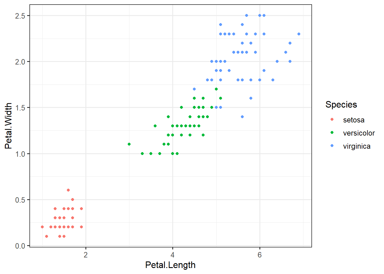
set.seed(20)
irisCluster <- kmeans(iris[,3:4], 3, nstart=20)
irisCluster
## K-means clustering with 3 clusters of sizes 52, 48, 50
##
## Cluster means:
## Petal.Length Petal.Width
## 1 4.269231 1.342308
## 2 5.595833 2.037500
## 3 1.462000 0.246000
##
## Clustering vector:
## [1] 3 3 3 3 3 3 3 3 3 3 3 3 3 3 3 3 3 3 3 3 3 3 3 3 3 3 3 3 3 3 3 3 3 3 3 3 3
## [38] 3 3 3 3 3 3 3 3 3 3 3 3 3 1 1 1 1 1 1 1 1 1 1 1 1 1 1 1 1 1 1 1 1 1 1 1 1
## [75] 1 1 1 2 1 1 1 1 1 2 1 1 1 1 1 1 1 1 1 1 1 1 1 1 1 1 2 2 2 2 2 2 1 2 2 2 2
## [112] 2 2 2 2 2 2 2 2 1 2 2 2 2 2 2 1 2 2 2 2 2 2 2 2 2 2 2 1 2 2 2 2 2 2 2 2 2
## [149] 2 2
##
## Within cluster sum of squares by cluster:
## [1] 13.05769 16.29167 2.02200
## (between_SS / total_SS = 94.3 %)
##
## Available components:
##
## [1] "cluster" "centers" "totss" "withinss" "tot.withinss"
## [6] "betweenss" "size" "iter" "ifault"table(irisCluster$cluster, iris$Species)##
## setosa versicolor virginica
## 1 0 48 4
## 2 0 2 46
## 3 50 0 0irisCluster$cluster <- as.factor(irisCluster$cluster)ggplot(iris,
aes(Petal.Length,
Petal.Width,
color=irisCluster$cluster)) +
geom_point()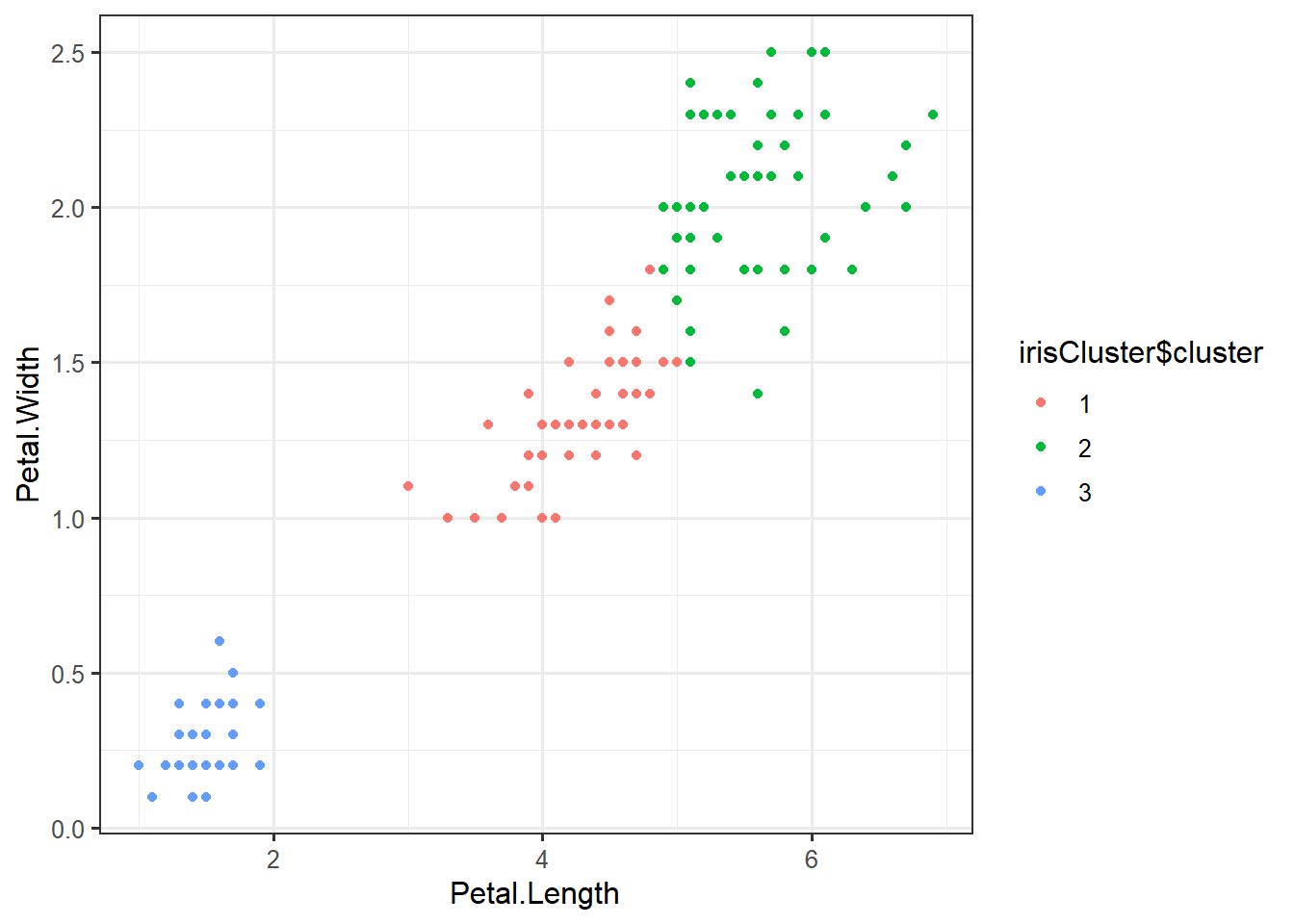
set.seed(1234)
x <- rnorm(12, mean=rep(1:3, each=4), sd=0.2)
y <- rnorm(12, mean=rep(c(1, 2, 1), each=4), sd=0.2)
plot(x, y, col="blue", pch=19, cex=2)
text(x + 0.05, y + 0.05, labels=as.character(1:12))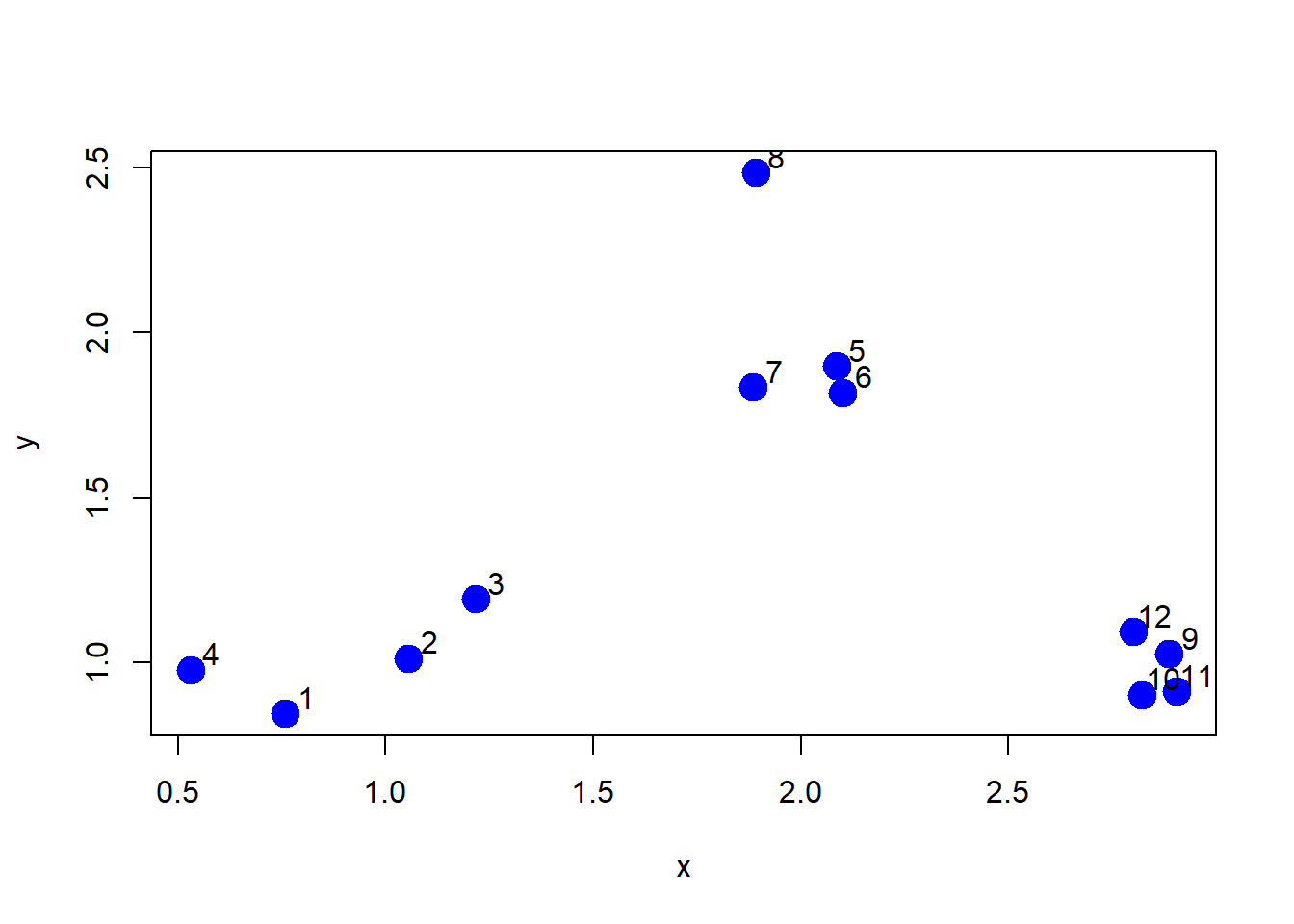
dataFrame <- data.frame(x, y)
kmeansObj <- kmeans(dataFrame, centers=3)
names(kmeansObj)
## [1] "cluster" "centers" "totss" "withinss" "tot.withinss"
## [6] "betweenss" "size" "iter" "ifault"kmeansObj$cluster## [1] 3 1 1 3 2 2 2 2 2 2 2 2par(mar=rep(0.2, 4))
plot(x,y, col=kmeansObj$cluster, pch=19, cex=2)
points(kmeansObj$centers, col=1:3, pch=3, cex=3, lwd=3)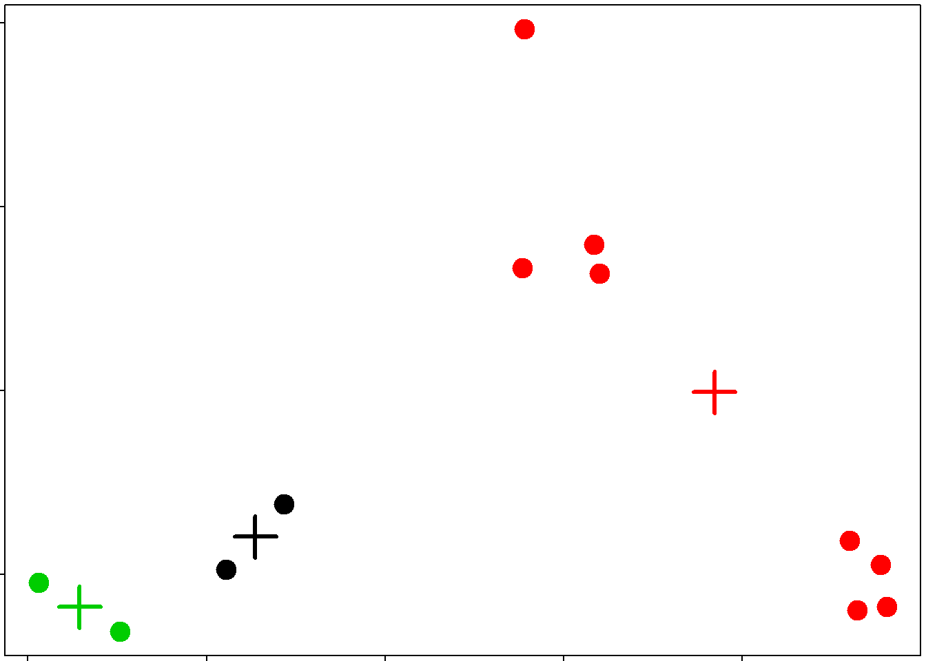
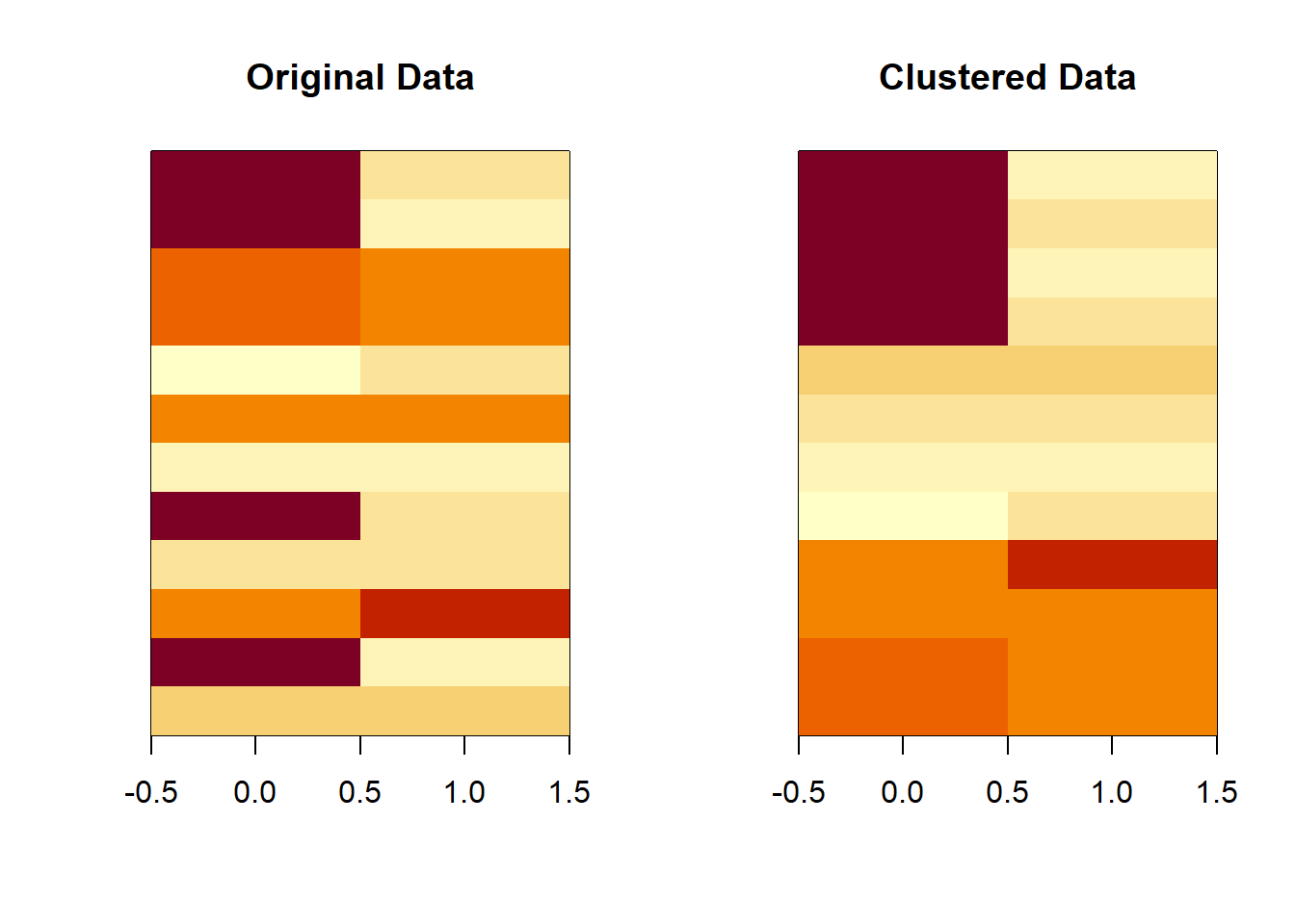
set.seed(1234)
dataMatrix <- as.matrix(dataFrame)[sample(1:12), ]
kmeansObj <- kmeans(dataMatrix, centers = 3)
par(mfrow = c(1, 2))
image(t(dataMatrix)[, nrow(dataMatrix):1], yaxt = "n", main = "Original Data")
image(t(dataMatrix)[, order(kmeansObj$cluster)], yaxt = "n", main = "Clustered Data")