Seedling Image Classification - A Convolutional Neural Network Problem in RStudio
Table of Contents
- The Project Origins
- Image Data
- The Data Science Problem
- The Software to Work the Problem
- Data Exploration
- Image Augmentation
- Base Model
- VGG16 Pretrained Model
- Training and Validation Graphs
- Data Augment – Balance Classes
- VGG16 Pretrained Model – Freeze/Unfreeze
- Training and Validation Graphs
- Predictions and Evaluations –VGG16
- Multi-Class ROC/AUC
- Improving the model - Part 2
- Predictions and Evaluations –VGG16
- Multi-Class ROC/AUC
- Summary
- References
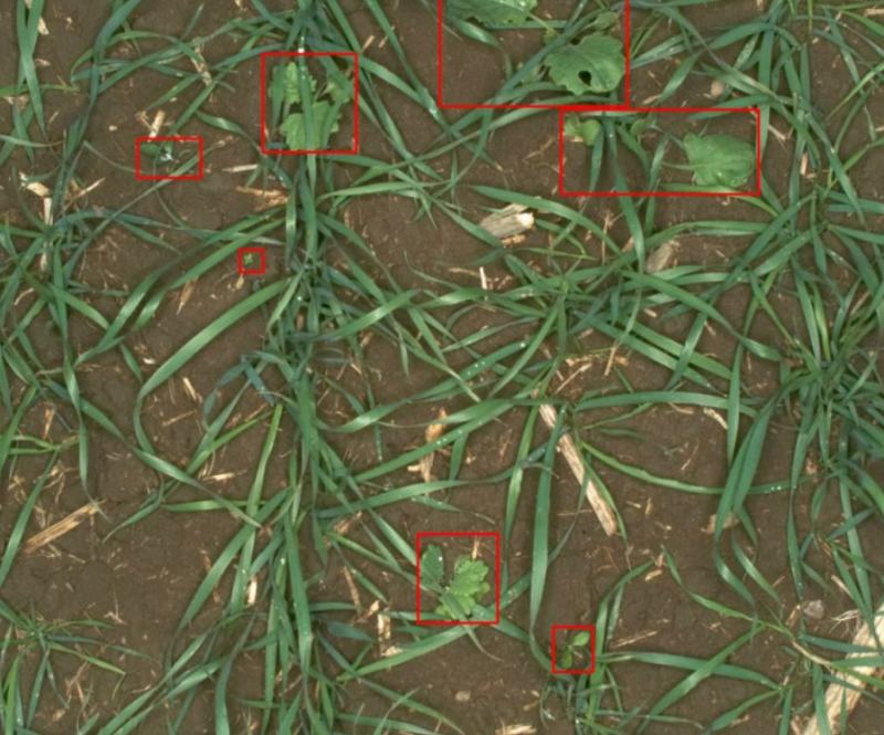
Figure 1: Image of invasive weed species growing in a crop. Image Source: https://vision.eng.au.dk/roboweedmaps/
Project Origins
Aarhus, Denmark, is one of the leaders in smart city research. The Aarhus University Computer Vision and Biosystems Signal Processing Group has been working on a project to use computer vision to detect seedlings of the weeds within crops and have made the dataset publicly available. The more significant implications of this problem benefit automated agriculture production. The need for this technology has immediate benefits for farmers because it will help to reduce the use of herbicides on the environment and to treat the invasive species before the weeds use all the available nutrients needed by the produced crop.
A camera mechanically scans the crops early in the growing season shortly after germination. The data can then be processed through an image classification model and output what species of early detected weeds are growing. Establishing a herbicide application plan to spray for the specific types of invasive plants will have benefits of not over-spraying chemicals into the environment, and product cost savings by reducing the amount and frequency of applications to crops.
The benefits are to the environment and the number of herbicides released into the atmosphere. Cost savings and increased productivity by doing other essential tasks for staff are the results of using only the specific amount and type of herbicide narrowed down to invasive plant type. The longer reaching benefit of the project is to automate agriculture with AI and autonomous systems.
- Computer Vision and BioSystems Signal Processing Group – Aarhus University, Denmark
- Detect Invasive Plants in Agriculture – Weeds take Soil Nutrients from the Produced Crop
- Reduction of Herbicides – Cost and Environment
- Automated/ Robotic Agriculture Production – Its the Future
This project will use a publically available dataset, and the images of seedlings will be classified using convolutional neural networks in Keras for R with TensorFlow back-end to classify 12 species of seedling growth images. I will use computer vision, deep learning techniques to solve this problem. This seedling image classification presentation will describe the problem and cover all the steps and observations taken to develop a working outcome leaving room for further testing.
Image Data
The data I collected is the plant seedling dataset. It is single plant cropped images and was a substantial file download at 1.7GB. The data file has 12 labeled folders of images for each weed species, and the images are PNG’s marked 1 to n per folder. There are five thousand five hundred and thirty-nine PNG images total. The images range in different pixel resolutions and sizes.
- Plant Seedlings Dataset – V2 Non-segmented Single Plants (Cropped Images) 1.7 GB File Size
- Retrieved from: Computer Vision and BioSystems Signal Processing Group Link: https://vision.eng.au.dk/plant-seedlings-dataset/
- 12 directories for each individual plant by species
- The folders labeled by plant name – Pictures in folders are labeled PNGs files. 1(n) for that plant type
- There are 5,539 PNG images total
- Different image size and resolutions
The Data Science Problem
The problem is to identify and classify the seedling images of weed species. It is a multi-class classification problem with 12 classes. We are dealing with large file size for a local computer environment. The image classification technique used will be the convolutional neural network and is a category of deep learning for computers. I chose the convolutional neural network because it is the most commonly used method to evaluate pictures and imagery at the time of this project.
- The problem is to identify and classify images of plant seedlings
- A multi-class image classification problem – 12 categories of images
- Large file size for a local computer environment
- Convolutional Neural Network (ConvNet or CNN’s) – A part of deep learning neural networks
- Convolutional Neural Networks are commonly used to evaluate the picture and video imagery
Software to Work the Problem
The software that I used is based in Rstudio. Keras is the leading deep learning library and has been available for just over a year for R as of this project implementation. However, available for Python longer. Under Keras is TensorFlow, Python, Virtual Studio. Nvidia CUDA and cuDNN is loaded because we can use my computers GTX1070 graphics card to do the neural network calculations. This project would not be possible without this support! This project will not discuss the in-depth process of setting the software up to run CNNs. Refer to the online documentation for Keras and its dependencies. The following software is all open-source, MS Visual Studio was used as a trial version.
- Rstudio™
- Keras™ Library – A Deep Learning Library Adapted to R High-Level Interface
- TensorFlow™ for R - Low-Level
- Anaconda Python™ 3.7
- MS Visual Studio™
- Nvidia CUDA™ Toolkit – GPU Support
- Nvidia cuDNN™ – GPU Support
Data Exploration
Exploring the image files as earlier mentioned 1.7GB with 12 directories labeled for each type of weed seedling species, the individual PNG’s are labeled 1(n). There are breaks in the numbering as if they deleted images at some point and image sizes vary greatly from 21 to 1700 pixel squares which may or may not affect model accuracy The images are mostly centered and cropped in tight but are also blurry, fuzzy, with irregular background from brown pebbles to a black and white striped scale from the lab where these images originate.
- 1.7GB
- 12 individual directories
- Each directory is labeled and has pictures numbered 1.png through 1(n).png
- The images in each folder have missing chronological numbering
- Image sizes vary (21x21px, 311x311px, 1700x1700px)
- Focus, blurry, skewed, irregular background (pebbles, b&w scale, etc.)
| 12 Categories | Total Number |
|---|---|
| Black Grass | 309 |
| Charlock | 452 |
| Cleavers | 335 |
| Common Chickweed | 713 |
| Common Wheat | 253 |
| Fat Hen | 538 |
| Loose Silky-Bent | 762 |
| Maize | 257 |
| Scentless Mayweed | 607 |
| Shepherd’s Purse | 274 |
| Small-Flowered Cranesbill | 576 |
| Sugar Beet | 463 |
The sampling of images shown. I scaled them all the same for this visual. One thing to note is for each seedling, there are several different growth stages from seedling to mature leaves. Note the background brown pebbles and some with the black and white striping. I am assuming the black and white striping is the edge of the container and may be used to scale the plants.
- 3 Samples
- 12 Categories
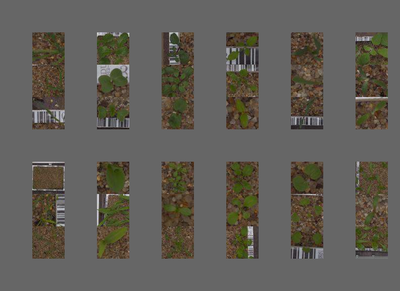
Figure 2: Top row, left to right: Black Grass, Charlock, Cleavers, Common Chickweed, Common Wheat, Fat Hen. Bottom row, left to right: Loose Silk-Bent, Maize, Scentless Mayweed, Shepherd’s Purse, Small Flowered Cranesbill, Sugar Beet.
- Class Imbalance
| Class Imbalance | Total Number | Percent of Total |
|---|---|---|
| Black Grass | 309 | 5.6% |
| Charlock | 452 | 8.2% |
| Cleavers | 335 | 6.0% |
| Common Chickweed | 713 | 12.9% |
| Common Wheat | 253 | 4.6% |
| Fat Hen | 538 | 9.7% |
| Loose Silky-Bent | 762 | 13.8% |
| Maize | 257 | 4.6% |
| Scentless Mayweed | 607 | 11.0% |
| Shepherd’s Purse | 274 | 4.9% |
| Small-Flowered Cranesbill | 576 | 10.4% |
| Sugar Beet | 463 | 8.4% |
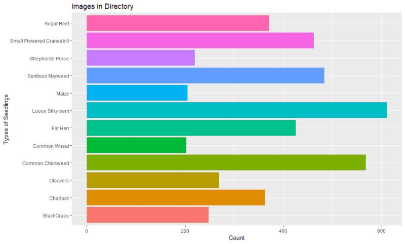
Figure 3: Here is a plot of the distribution of the 12 classes. From 253 of the common wheat to 762 of the Loose Silky-bent. The first impression is this will be an unbalanced classification problem.
I begin with splitting the images into 80% training 10% validation and 10% testing folders. The validation set is used to pre-test the CNN because if we do multiple runs on the test set, these models will leak and pick up information from the test set over time. With the validation set, the model never sees the fresh new test data. CNN’s need large numbers of images to train the model. 10’s of thousands of images are ideal. Large file size of image data is not optimal for this project, and this is a small dataset for my processing environment.
- 80% training – 4475 images
- 10% validation – 552 images
- 10% test – 562 images
- Validation and Test Set Class Proportions
table(factor(train_generator$classes))
| Class | Training Quantity |
|---|---|
| 0 | 247 |
| 1 | 362 |
| 2 | 268 |
| 3 | 567 |
| 4 | 202 |
| 5 | 424 |
| 6 | 611 |
| 7 | 204 |
| 8 | 483 |
| 9 | 219 |
| 10 | 461 |
| 11 | 370 |
table(factor(validation_generator$classes))
| Class | Validation Quantity |
|---|---|
| 0 | 31 |
| 1 | 46 |
| 2 | 34 |
| 3 | 72 |
| 4 | 26 |
| 5 | 55 |
| 6 | 75 |
| 7 | 26 |
| 8 | 61 |
| 9 | 28 |
| 10 | 59 |
| 11 | 47 |
table(factor(test_generator$classes))
| Class | Test Quantity |
|---|---|
| 0 | 32 |
| 1 | 44 |
| 2 | 33 |
| 3 | 74 |
| 4 | 25 |
| 5 | 59 |
| 6 | 76 |
| 7 | 25 |
| 8 | 63 |
| 9 | 27 |
| 10 | 56 |
| 11 | 46 |
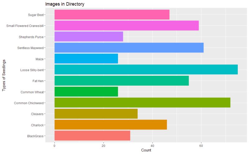
Figure 4: Validation and Test Set Class Proportions. Randomized samples of 10% Validation 10% Test
Image Augmentation
Image augmentation addresses the issue of small data in CNN training. By using’s Kera’s Image Data Generator, I can create altered copies of existing images by shifting, skewing, flipping, scaling, and rotating an existing image. These are random transformations to the images to help train the CNN on more instances of different versions of the same pictures.
- Too few samples to train – Random transformations to random images
- The model will see more variations of the images
- Rotate 40 deg,
- Shift left/right by 0.2, shift up/down by 0.2,
- Zoom by 0.2,
- Shear (tilt) by 0.2
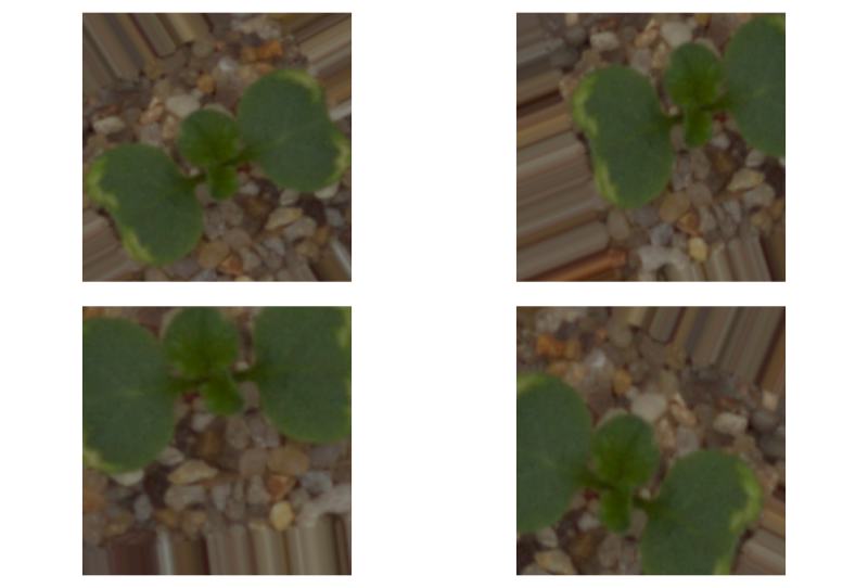
Figure 5: Top row image is shifted right. Bottom row shows image rotated couter clockwise and shifted up.
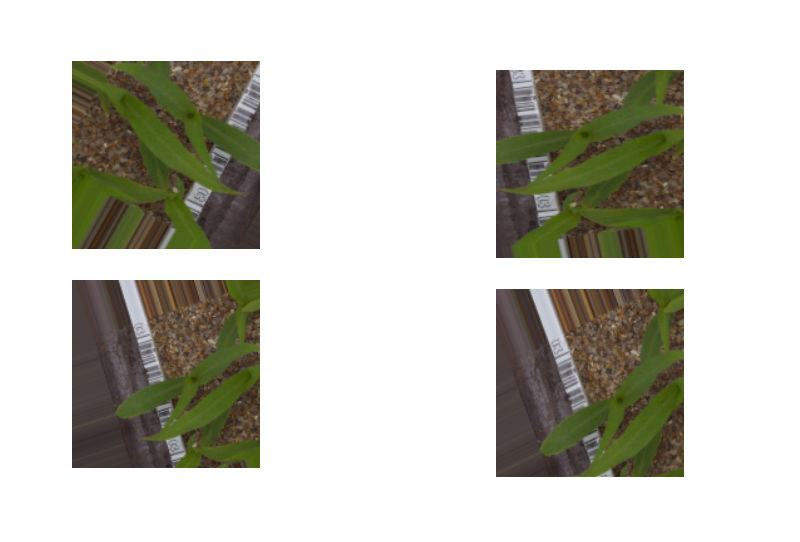
Figure 6: Top row image is rotated clockwise. Bottom row the image is shifted downward.
Base Model
Shown is the base CNN model. It is layers of tensors stacked together, and the network works over each layer. It starts with a specified image size and color channel and decreases in a densely connected layer holding only the parameters that define each of the 12 classes. This model goes through 3.4 million parameters. It starts with 148 x 148-pixel images. The third number is the RGB color channel.
Basic ConvNet:
- A stack of layers
- The shape is the image size and decreases
- The last layer has 12 outputs for 12 classes
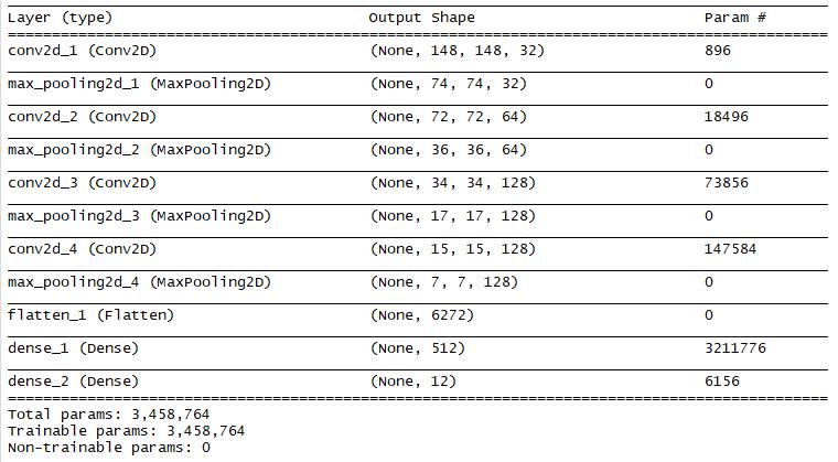
Figure 7: The base model tensors shown in Keras for RStudio.
VGG16 Pretrained Model
In contrast, this is a VGG16 pertained model used in this project. This model is loaded from Keras and pre-trained on 1000+ image categories. Note the flattening and dense layers not included. Alone this model has 14.7 million parameters that are calculated over and start with 299 x 299 squared pixeled images.
- Trained on Image Net 1000’s of classes:
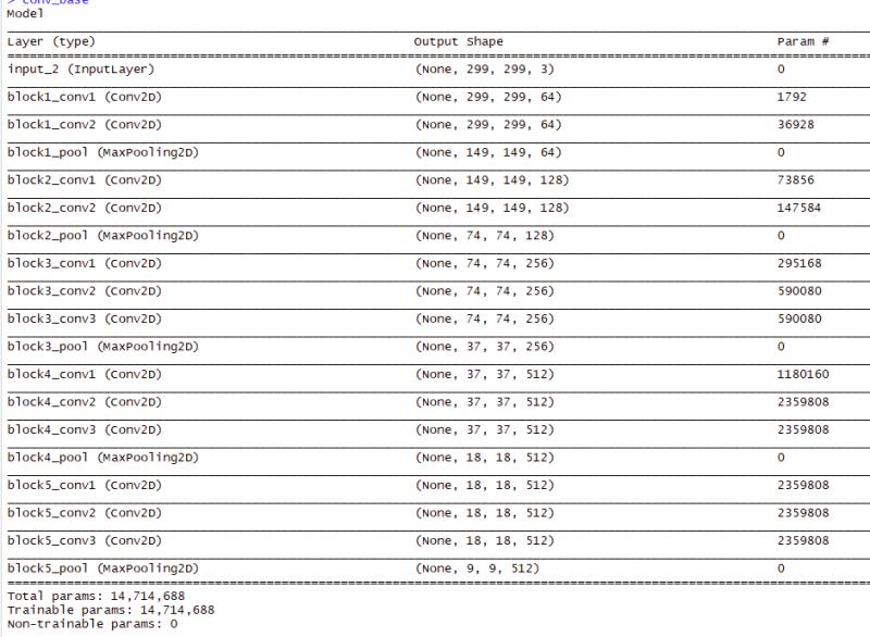
Figure 8: The parameters shown for the VGG16 model
VGG16 Training and Validation
I ran the early training with the base model first. The first graph demonstrates the results of using the data as-is with no extra steps. We see the training data is overfitting, and the loss function is higher. The second model shows what happens when I added the random image augmentation and added a dropout layer to reduce overfitting The drop out is a regularization technique that randomly sets some output features to zero. What we need to know is it reduces overfitting of the model. And in the second graph, we can see the training and validation are much closer. The area between 15 and 20 epochs is where the model fits well, but accuracy is still too low.
- Training Accuracy = 86.6%
- Validation Accuracy = 76%
- Overfitting
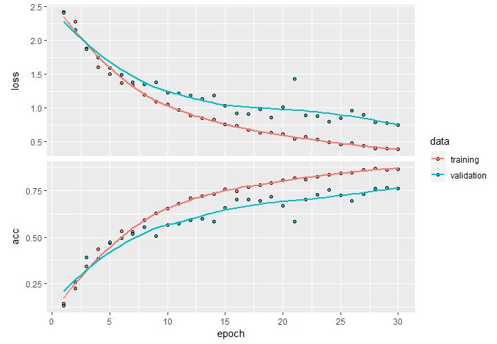
Figure 9: The graph shows overfitting of the model, the blue and red lines diverge early and the distance increases at 30 epochs.
- Training Accuracy = 69%
- Validation Accuracy = 66.6%
- Added Dropout Augmentation = Reduce Overfit
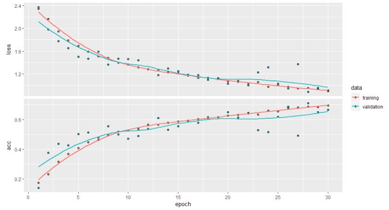
Figure 10: The graph shows reduced overfitting of the model, the blue and red lines converge earlier, epoch 16-18, then drift apart. However, still closer then the previous run of the model
Here is the VGG16 model; this one uses the base layers with 25.3 million parameters. The process is to add my network on top of the already trained VGG16. I freeze the base network first, train the part I added. Unfreeze some layers in the base above and jointly train both of these layers and the part I added.
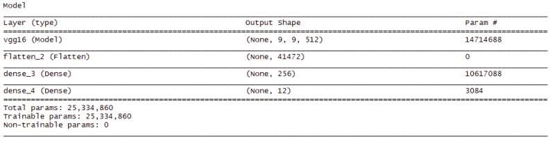
Figure 11: VGG16 Pretrained Model Freeze/Unfreeze. Note the 25M params.
Figure 12 may show low accuracy but is fitting well and very little overfitting. Figure 13 shows the unfrozen layer, and my layers added for a longer training run of 100 epochs The accuracy has increased to 96.7 and 95.2 percent. I see it is overfitting at around 1.5%, but not sure why.
VGG16 freeze base layers:
- Training Accuracy = 57.3%
- Validation Accuracy = 57%
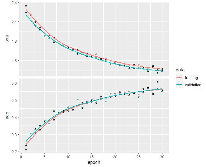
Figure 12: VGG16 - Freeze base layers. 150x150.
VGG16 unfreeze base layers:
- Training Accuracy = 96.7%
- Validation Accuracy = 95.2%
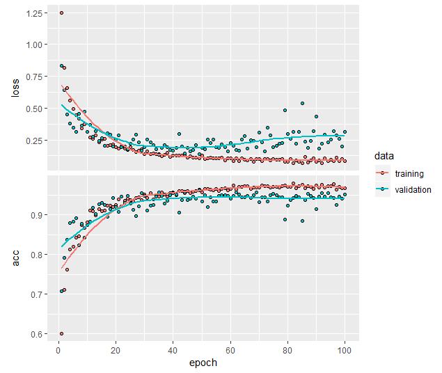
Figure 13: VGG16 - Unfreeze base layers. 150X150.
Predictions and Evaluations – VGG16
I run a prediction on my test data now. To validate this model, I create a confusion matrix from the predicted and test labels. 87.8% accuracy with a Kappa of 0.86 isn’t too bad but not great.
VGG16 Prediction:
- Predicted Accuracy = 87.8%
- Kappa = 0.866
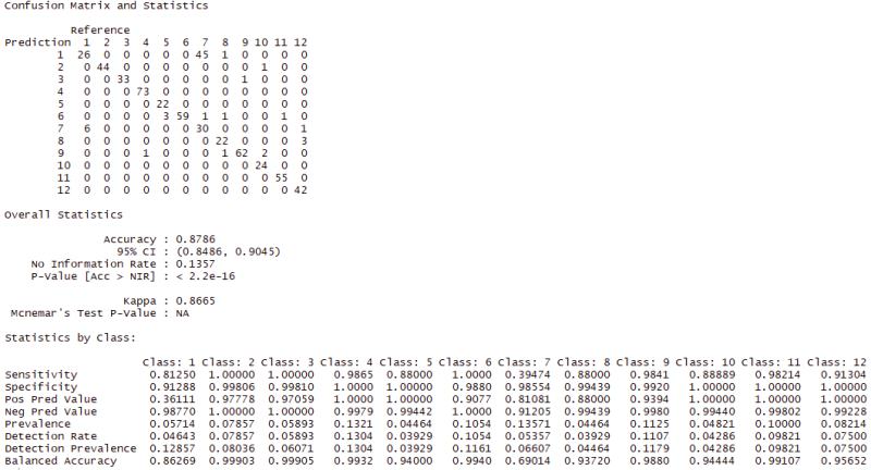
Figure 14: VGG16 Unfreeze 150x150. Confusion Matrix
In the matrix, I see 45 False Positives (FP) for the Loose Silky-Bent, and it looks like that is pulling the overall accuracy down. Not sure as to why this happened.
False Positive:
- 45 false positives of class 7 - Loose Silky-Bent
Image comparision of the mis-classified Loose Silky-Bent. 69% balanced accuracy with a 39.4% sensitivity. Figure 15 shows the two classes top and bottom. This makes sense why the model would think one is the other because they look similar.
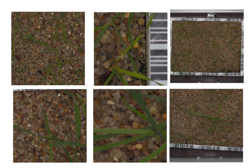
Figure 15: Top row is Loose Silky-Bent. The model produced 45 False Positves mistaken for the Blackgrass on bottom row. Both are very similar with the narrow green leaves.
Multi-Class ROC/AUC
I evaluate the model results using the mean Reciever Operating Characteristics (ROC) curve and the mean Area Under the Curve (AUC) because it is a multi-class problem. This model did reasonably well with an AUC of 93.1%. The prediction is reliable, but the model needs work to bring the accuracy up.
- Mean AUC = 93.12%
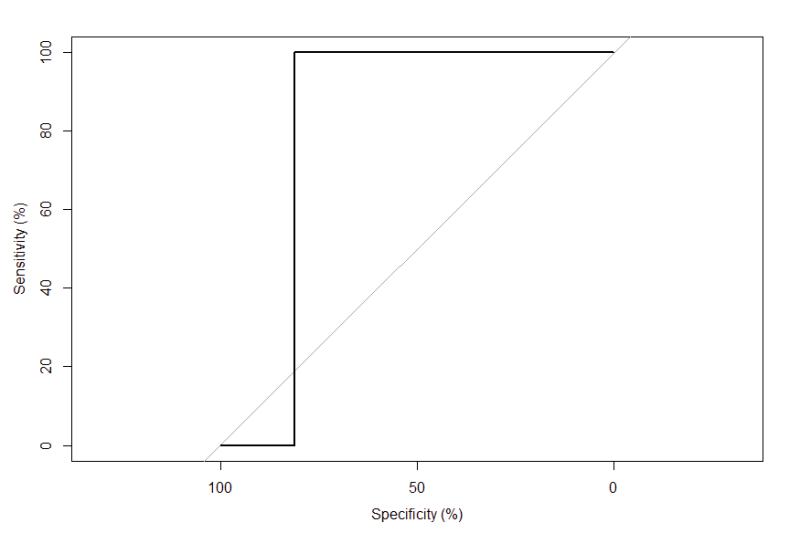
Figure 16: Mean AUC is 93.1% using the 150x150 VGG16 unfreeze model.
Classes Close to 0,1:
- Class 7 69%
- 12 Classes ROC Plot
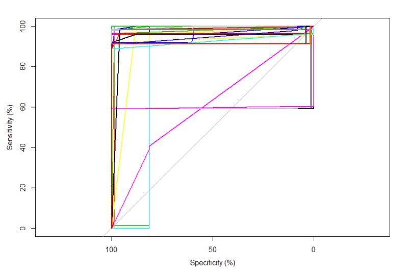
Figure 17: The graph shows each individual ROC and as the matrix tables showed the majority are close or at 0,1. The magenta colored line cutting across is class 7.
Improving model - Part 2
After running the baseline and observing the results, there is room to make the model better. I found that the class imbalance could be an issue with CNN’s. I augmented random samples of images in each of the training directories to bring the image counts up to the 610 each to that of the Loose-Silk-bent class. I applied randomly different augmenting parameters to the pictures using the image data generator in Keras, which has 17 different ways to change the images. Now I have a balanced dataset to test the model further.
- Data Augmentation – Balance Classes Use the image augmentation technique
- Randomly augment all other classes to bring to 610 for each class
- Keep the max quantity of 610 for Loose Silky-Bent
table(factor(train_generator$classes))
| Class by Name | Training Quantity |
|---|---|
| Black Grass | 247 |
| Charlock | 362 |
| Cleavers | 268 |
| Common Chickweed | 567 |
| Common Wheat | 202 |
| Fat Hen | 424 |
| Loose Silky-Bent | 611 |
| Maize | 204 |
| Scentless Mayweed | 483 |
| Shepherd’s Purse | 219 |
| Small-Flowered Cranesbill | 461 |
| Sugar Beet | 370 |

Figure 18: Showing the before augmentation and imbalanced data
table(y)
| Class by Name | Augmented Number |
|---|---|
| Black Grass | 610 |
| Charlock | 610 |
| Cleavers | 610 |
| Common Chickweed | 610 |
| Common Wheat | 610 |
| Fat Hen | 610 |
| Loose Silky-Bent | 610 |
| Maize | 610 |
| Scentless Mayweed | 610 |
| Shepherd’s Purse | 610 |
| Small-Flowered Cranesbill | 610 |
| Sugar Beet | 610 |
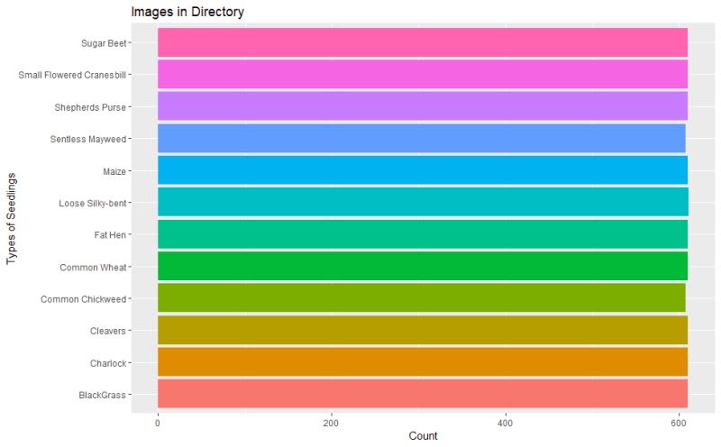
Figure 19: Augmented data to bring each class up in numbers so there is more data to train the models.
I am going back to the base model again, but this time I have a balanced data set, and I have increased the size of the images to 299 x 299 pixels. More pixels to process, maybe more detail for the model to grab? The graph on the left shows overfitting but improved accuracy of 92.3% and slightly improved validation accuracy of 77.8% over the earlier run with imbalanced data. Figure 21 shows the overfitting reduced, and accuracy is up to 70% while the validation accuracy is up to 74% over the baseline imbalanced data.
Training and Validation Graphs
- Balanced Data @ 299 x 299 pixel images Freeze
- Overfitting
- Training Accuracy = 92.3%
- Validation Accuracy = 77.8%
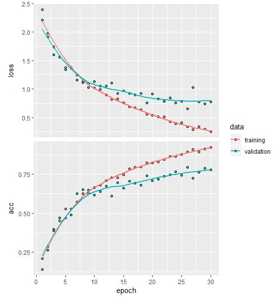
Figure 20: Overfitting on the balanced data and increased the pixel size to 299 x 299.
- Reduced overfitting
- Training Accuracy = 70%
- Validation Accuracy = 74.1%
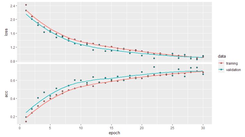
Figure 21: Overfitting reduced.
The graph shows the unfrozen layer with my layers added for a longer training run of 100 epochs up from 30 epochs. The final training model. The accuracy has increased again over the baseline to 97.3% accuracy and 95.5% validation accuracy (same as before). I see it is overfitting around 2%, but not sure at this point.
Training and Validation Graphs
- Balanced Data @ 299 x 299 pixel images UnFreeze
- Training Accuracy = 97.3%
- Validation Accuracy = 95.5%
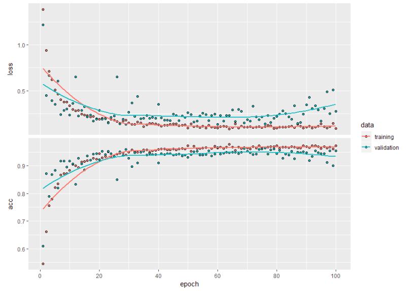
Figure 22: Model unfreezed on 299 x 299 pixels, shows overfitting again.
I run the prediction on the test set with this new model. I am pleased to see an increase in model Accuracy of 92% and Kappa to 91%. I now have a False Negative amount of 22 in Class 1, but it is related to Class 7 from before where there was a FP of 45. Looking through the table at the bottom, a balanced accuracy of 64.7% for class 1, the Black Grass, and it looks like this is bringing down the overall model accuracy, which could be much higher. I think I know why, but let us look at the ROC and AUC for this model.
Predictions and Evaluations – VGG16
VGG16 Prediction:
- Predicted Accuracy = 92.1%
- Kappa = 0.913
False Negative:
- Class 1 – Black Grass
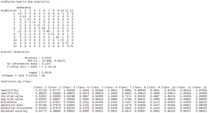
Figure 23: Confusion Matrix results on the test data.
The mean area under the curve has improved to 94.9%, almost a 2% improvement from earlier. It seems like the model is working as designed for the most part.
Multi-Class ROC and AUC
Multi-class area under the curve (AUC) = 94.9%
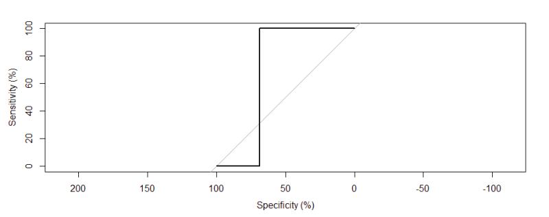
Figure 24: Reciever Operating Characteristics (ROC). Area Under the Curve (AUC) = 94.9%
In figure 25 we can see how the majority of classes are close to 0,1 while Class 1 is 64%.
Multi-Class ROC:
- Majority of Classes close to 0,1
- Class 1 @ 64%
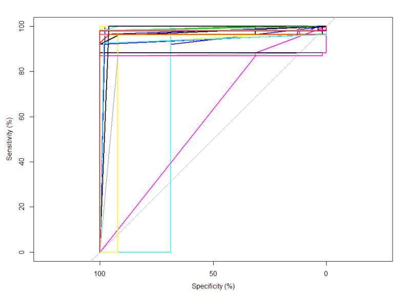
Figure 25: ROC curve. Magenta line is Class 1 and at 64% AUC.
Summary
For this multi-class classification problem, we can predict and classify images from 12 categories to varying degrees of accuracy. From the model steps, the smaller image size and imbalanced data produced fairly decent results of 87.8% percent and an AUC of 93.1% After adding more augmented images to balance the data to 610 for each class and increasing the image size, I re ran the models and increased the accuracy to 92.1% and increased the reliability of the model with an AUC of 94.1%. I placed the images of class 7 and class 1 the loose silky-bent and the black grass together previously in figure 15, and they look very similar, explaining the misclassification in both models.
I think the next step is to use further image augmenting techniques to highlight what makes each grass unique I would like to see if I can mask the background to remove the pebbles and black and white bar. At the time of this project, I couldn’t find a method in R to do this until yesterday and can potentially use a library called OpenImageR but entirely not sure if I can batch process this to all images. I think masking the image background will be the next step to improving this model.
- Multi-Class Classification of 12 categories of seedling images
- Using pre-trained Convnet VGG16 architecture trained on ImageNet as the base layers
VGG16 Prediction
Imbalanced Train Set @ 150 x 150 pixels
- Predicted Accuracy = 87.8%
- Kappa = 0.866
- Mean AUC = 93.12%
- False Positive Class 7 - Loose Silky-Bent
| Predicted /Labeled | Black Grass | Charlock | Cleavers | Common Chickweed | Common Wheat | Fat Hen | Loose Silky-Bent | Maize | Scentless Mayweed | Shepherd’s Purse | Small-Flowered Cranesbill | Sugar Beet |
|---|---|---|---|---|---|---|---|---|---|---|---|---|
| Black Grass | 26 | 0 | 0 | 0 | 0 | 0 | 45 | 1 | 0 | 0 | 0 | 0 |
| Charlock | 0 | 44 | 0 | 0 | 0 | 0 | 0 | 0 | 0 | 1 | 0 | 0 |
| Cleavers | 0 | 0 | 33 | 0 | 0 | 0 | 0 | 0 | 1 | 0 | 0 | 0 |
| Common Chickweed | 0 | 0 | 0 | 73 | 0 | 0 | 0 | 0 | 0 | 0 | 0 | 0 |
| Common Wheat | 0 | 0 | 0 | 0 | 22 | 0 | 0 | 0 | 0 | 0 | 0 | 0 |
| Fat Hen | 0 | 0 | 0 | 0 | 3 | 59 | 1 | 1 | 0 | 0 | 1 | 0 |
| Loose Silky-Bent | 6 | 0 | 0 | 0 | 0 | 0 | 33 | 0 | 0 | 0 | 0 | 1 |
| Maize | 0 | 0 | 0 | 0 | 0 | 0 | 0 | 22 | 0 | 0 | 0 | 3 |
| Scentless Mayweed | 0 | 0 | 0 | 0 | 0 | 0 | 0 | 0 | 62 | 2 | 0 | 0 |
| Shepherd’s Purse | 0 | 0 | 0 | 0 | 0 | 0 | 0 | 0 | 0 | 24 | 0 | 0 |
| Small-Flowered Cranesbill | 0 | 0 | 0 | 0 | 0 | 0 | 0 | 0 | 0 | 0 | 55 | 0 |
| Sugar Beet | 0 | 0 | 0 | 0 | 0 | 0 | 0 | 0 | 0 | 0 | 0 | 42 |
VGG16 Prediction
Balanced Train Set @ 299 x 299 pixels
- Predicted Accuracy = 92.1%
- Kappa = 0.913
- Mean AUC = 94.12%
- False Positive Class 1 – Black Grass
| Predicted /Labeled | Black Grass | Charlock | Cleavers | Common Chickweed | Common Wheat | Fat Hen | Loose Silky-Bent | Maize | Scentless Mayweed | Shepherd’s Purse | Small-Flowered Cranesbill | Sugar Beet |
|---|---|---|---|---|---|---|---|---|---|---|---|---|
| Black Grass | 10 | 0 | 0 | 0 | 0 | 0 | 9 | 0 | 0 | 0 | 0 | 0 |
| Charlock | 0 | 43 | 0 | 0 | 0 | 0 | 0 | 0 | 0 | 0 | 0 | 0 |
| Cleavers | 0 | 1 | 33 | 0 | 0 | 1 | 0 | 0 | 0 | 0 | 0 | |
| Common Chickweed | 0 | 0 | 0 | 74 | 0 | 0 | 0 | 0 | 0 | 1 | 0 | 0 |
| Common Wheat | 0 | 0 | 0 | 0 | 23 | 0 | 1 | 1 | 0 | 0 | 0 | 0 |
| Fat Hen | 0 | 0 | 0 | 0 | 0 | 58 | 0 | 0 | 0 | 0 | 0 | 0 |
| Loose Silky-Bent | 22 | 0 | 0 | 0 | 2 | 0 | 66 | 1 | 0 | 0 | 0 | 1 |
| Maize | 0 | 0 | 0 | 0 | 0 | 0 | 0 | 22 | 0 | 0 | 1 | 0 |
| Scentless Mayweed | 0 | 0 | 0 | 0 | 0 | 0 | 0 | 1 | 62 | 1 | 0 | 0 |
| Shepherd’s Purse | 0 | 0 | 0 | 0 | 0 | 0 | 0 | 0 | 1 | 25 | 0 | 0 |
| Small-Flowered Cranesbill | 0 | 0 | 0 | 0 | 0 | 0 | 0 | 0 | 0 | 0 | 55 | 0 |
| Sugar Beet | 0 | 0 | 0 | 0 | 0 | 0 | 0 | 0 | 0 | 0 | 0 | 45 |
References
Aarhus University. (2018). Plant seedlings dataset. Retrieved from: https://vision.eng.au.dk/plant-seedlings-dataset/
Allaire, J., Chollet, F. (2018). Deep learning with R. (pp.111-148). Manning
Allaire, J. (2017). Using a pre-trained convnet. Retrieved from: https://jjallaire.github.io/deep-learning-with-r-notebooks/notebooks/5.3-using-a-pretrained-convnet.nb.html#
Brownlee, J. (2016). Image augmentation for deep learning with Keras. Retrieved from: https://machinelearningmastery.com/image-augmentation-deep-learning-keras/
Hodnett, M., Wiley, J. (2018). R deep learning essentials. Retrieved from: https://lumen.regis.edu/record=b1847282~S3
Keras. (2018). Reference. Retrieved from: https://keras.rstudio.com/reference/index.html
Lui, Y. (2018). R deep learning projects: master the techniques to design and develop neural network models in R. Retrieved from: https://lumen.regis.edu/record=b1816355~S3
Prakash, A., PKS. (2017). R deep learning cookbook: solve complex neural net problems with TensorFlow, H2O, and
MxNet. Retrieved from: https://lumen.regis.edu/record=b1787602~S3 Soumendra, P. (2018). [Keras] A thing your should know about Keras if you plan to train a deep learning model on a large dataset. Retrieved from: https://medium.com/difference-engine-ai/keras-a-thing-you-should-know-about-keras-if-you-plan-to-train-a-deep-learning-model-on-a-large-fdd63ce66bd2
TensorFlow for R. (2018). Tutorial: Overfitting and underfitting. Retrieved from: https://tensorflow.rstudio.com/keras/articles/tutorial_overfit_underfit.html
TensorFlow for R. (2018). Image classification on small datasets with Keras. Retrieved from: https://blogs.rstudio.com/tensorflow/posts/2017-12-14-image-classification-on-small-datasets/
Vijayabhaskar, J. (2018). Tutorial on using Keras flow_from_directory and generators. Retrieved from: https://medium.com/@vijayabhaskar96/tutorial-image-classification-with-keras-flow-from-directory-and-generators-95f75ebe5720